Ultimately, our
goal for behavior analysis is to predict fully the behavior that will
be supported by any given environment. The endpoint of our report's
data reduction is a c² assessment of a prediction of
steady-state dynamic behavior made by linear analysis. In the course
of this report, we will develop the techniques used for the
predictions and obtain some useful intermediate results.
Over the past
few decades, environmental input and the supported behavior have
often been characterized with globally time-averaged parameters.
Typically, reinforcement schedule data from an entire session, or
several sessions, are combined to yield a single parameter such as
average rate of reinforcement or average ratio of reinforcers between
the alternatives of a concurrent schedule. Similarly, long samples of
the supported behavioral output are compressed into a parameter such
as average responses per second or average ratio of responding
to the alternatives of a concurrent schedule.
This has been a fruitful approach and has led to quantitative molar
predictions for the dependence of global time average response rates
upon global time average schedule parameters. For at least some
schedules, these relationships are reasonably well established (e.g.,
the generalized matching law, Baum, 1979). The moment-to-moment
structure of behavior seen in response to a dynamic (i.e., time
varying) input, even in average steady state, has received less
attention.
Galbicka,
Kautz, and Jagers (1993) and Galbicka (in press) suggest that the
analysis of behavior be broadened well beyond contingencies that are
designed to
minimize local variation
in response structure (e.g., constant-probability variable-interval
schedules). The present report focuses on the steady-state behavioral
adaptation supported by an unsignaled step transition in the
contingencies of reinforcement and on describing this adaptation with
a linear analysis (McDowell, Bass, & Kessel, 1993). This focus on
the steady-state behavior supported by a schedule transition in
repeated trials provides an intermediate step between completely
local, or molecular, measurements of a unique behavioral occurrence
and global, or molar, time averages of behavior across multiple
sessions.
This experiment
has a very simple dynamic structure as part of the reinforcement
contingency: a step transition from a variable-interval (Vl) schedule
to extinction. Like a mixed schedule, the procedure repetitively
switched between a Vl schedule and extinction with no change in the
explicit stimuli. The task of the present research is not simply to
determine if pigeons peck during the period when the reinforcer is
available and refrain from pecking during extinction. Rather, our
task is to quantify the relation between this dynamic reinforcement
schedule and the supported behavior using a construct from linear
analysis called a transfer
function. (Note that
linear analysis, by itself, does not determine what schedule will be
the most useful in an initial study of behavioral dynamics.)
McDowell, Bass, and Kessel (1992) showed that if the transfer
function (or linear kernel) were known, then the dynamic behavior
supported by a step transition between two Vl schedules could be
computed. Of course, at present, the transfer function is not known a
priori; instead, it must be measured experimentally: If the average
moment-to-moment behavior generated by a particular step transition
is measured, then a computational technique exists that combines the
reinforcement schedule with the behavioral data to determine the
transfer function. Once an organism's transfer function is extracted
using one reinforcement input/behavior output pair, its behavior for
a new reinforcement schedule can he predicted based solely on this
transfer function and the new schedule. The more closely the
predicted behavior agrees with the measured behavior, the more useful
a linear analysis will be in understanding the relation between the
reinforcement schedule and supported behavior. Because this is the
first use of a linear analysis with time-dependent behavioral data, a
major portion of this paper is, accordingly, a presentation of the
analytic and numerical techniques involved.
The report
begins with the traditional description of the experimental method.
The next section then develops the general method and auxiliary
techniques we use to make a prediction of behavior. The first portion
of this section is an averaging method that is used to combine data
from the repeated trials. The second part is an introduction to
Fourier transforms (a standard technique of linear analysis). The
third subsection is a long thoroughgoing discussion of the method
used to extract a transfer function from data and predict behavior
under a new schedule. There are two parts in the results section.
First, we show, for 1 bird, all of the intermediate results obtained
in the process of determining the transfer function and predicting
the output given a novel input. In the second part of the results
section we define the appropriate reduced c² test and
then assess the predictions' fidelity to the observed behavior on the
new schedule for the remaining 15 birds. The paper concludes with a
brief discussion section. There is also an Appendix that covers some
relevant technical aspects of linear analysis.
METHOD
Subjects
Sixteen adult
experimentally naive pigeons obtained from a local supplier were
used. They were housed under a 19:5 hr light/dark cycle in individual
cages with free access to water. All were maintained at approximately
80% of their ad lib weights by limited feeding with pelletized laying
mash.
Apparatus
Five
experimental chambers were used. The interior of each was a box (30
cm by 30 cm by 34 cm high). An unfinished aluminum panel served as
one wall of the chamber; the other sides were painted white. The
stimulus panel had a feeder aperture 5 cm in diameter, medially
located 10 cm above the grid floor. Three response keys, each 2 cm in
diameter, were located 9 cm apart, 29 cm above the grid floor. Only
the center key was used. It required approximately 0.15 N to operate.
The key was transilluminated by a stimulus projector containing the
Rosco pea (86, yellow green) theatrical gel throughout all phases of
the experiment, with the exception of the scheduled blackouts and
during reinforcement. Two houselights were located on the stimulus
panel 32 cm above the grid floor. The lamps were shielded such that
their light was directed towards the ceiling. Ventilation was
provided by an exhaust fan mounted on the outside of the chamber. A
white noise generator provided ambient masking noise in the chamber.
Stimulus events were controlled and key pecks were recorded by a
computer system (Palya & Walter, 1993). The computer archived the
time of each stimulus and response event in 1-ms "ticks." Subsequent
data extraction and analysis routines provided the derived data.
Complete raw data event logs of all research are maintained for 10
years and are available from the authors.
Procedure
All pigeons
were magazine trained to approach and eat from the food magazine
within 3 s on three consecutive presentations. The birds were then
autoshaped to peck the center key, and subsequent responding was
maintained under a short Vl schedule in the presence of the
pea-colored keylight. To maintain a constant weight throughout the
course of the experiment, each session typically contained 45 to 55
food presentations, the exact number being determined by the bird's
body weight that day. Experimental treatments (phases) were continued
until there were no apparent session-to-session trends in the data,
as judged by visually inspecting daily plots of behavioral measures.
The data came
from two Vl-to-extinction step-transition schedules (Phases 1 and 2).
The step-transition procedure is illustrated in Figure 1. Within each
trial, the pigeons were first exposed to a Vl schedule for a period
Tvi Next, an unsignaled transition to extinction occurred. There were
no changes in any explicit stimuli. Extinction was in effect from Tvi
to Ttrial The only stimulus correlated with the step transition was
the consistent temporal duration of Tvi The end of the extinction
period was followed by a 10-s blackout, during which the chamber was
totally dark. This blackout procedure provided a relatively sharp
demarcation at the beginning of each trial. The chamber was also dark
for several seconds between the time the birds were first put in the
chamber and the time the control software started a session's first
trial. There were typically five step- transition trials in each
session.

Fig. 1. A
schematic of the basic procedure used for the transition trials of
this experiment. The time intervals used are Ttrial = 1,000 s, a 10-s
chamber blackout, and Tvi = 200 s or 300 s. R(t)) is the locally
averaged reinforcement rate.
Any initial
study of steady-state behavioral dynamics necessarily has an
exploratory character. Because the stability and orderliness of the
supported behavior were unknown at the outset of the experiment, we
exposed 8 birds to the procedures with Vl schedules composed of
exponential (Fleshier & Hoffman, 1962) distributions of
interreinforcement intervals (IRI). A second set of 8 birds had
rectangular IRI distributions. Our selections for Phase 1 were a V1
20-s schedule with Tvi of 200 s followed by 800 s of extinction,
yielding a Ttrial of 1,000 s. During Phase 2, we grouped the birds
into sets of 4 and changed either the Tvi (200 s to 300 s) or the Vl
schedule (V1 20 s to V1 40 s) so we could test the predictions of
linear analysis. Ttrial was held constant for computational ease. The
average number of reinforcers was determined by the trial duration
and the Vl schedule. The actual Vl schedules were constructed with a
sequence of IRI times that were exhaustively drawn, without
replacement, from a randomized pool containing five sets of identical
20 element Fleshler- Hoffman or rectangular values (i.e., similar to
a Vl tape). Each experimental session was begun at a random point in
that fixed sequence of IRI times.
CONCEPTUAL
FRAMEWORK AND
AUXILIARY
TECHNIQUES
Determining the
quantitative relationship between the obtained structure in
steady-state behavior and the supporting reinforcement schedule is
the core of our linear analysis. There are two auxiliary techniques
that are required to obtain and use this relationship— one
specialized for repeated-trials data and the other quite general. We
will cover these auxiliary techniques first and then subsequently
address the framework used to predict behavior.
Averaged
Steady-State Dynamics
This subsection
defines the technique that we used to obtain an average steady state
from the repeated- trials data. The characteristics of the average
are briefly discussed. In addition, we will consider the resulting
averages without reference to linear analysis.
We applied a
technique, the repeated-trials local average,
to both the input data
(reinforcer delivery times) and the output data (operant response
times) to combine the steadystate trials. This is a common technique
used to compute the average behavior supported by a fixed-interval
(FI) schedule: The within-trial elapsed time for a set of trials is
first synchronized to a common time base and the resulting ensemble
is then averaged. For this experiment's data reduction we used a
common time base, Ttrial in length, divided into 512 equal time
subintervals, or bins. The reinforcement and response times from all
trials after stability occurred (as noted, the final 20 sessions)
were mapped to the common time base. We computed the local average
rates of reinforcement and responding for each bin by dividing the
number of events occurring in the bin by the time duration of that
bin. The end result is the averaged moment-to-moment changes in the
reinforcement rate and the response rate at each point in the trial
interval. The choice of 512 bins was determined by the fast Fourier
transform (FFT) routines used in the linear analysis.
A
repeated-trials local average condenses the completely local (or
molecular) snapshots of behavior or reinforcement from the individual
trials into a single composite picture. To reach the more global time
averages used in molar studies, one would continue condensing the
data along the length of the common time-base interval by further
averaging across the 512 bin rates to produce a single average rate.
A repeated-trials local average is probably meaningful only after an
organism has reached steady state. Furthermore, the obtained
repeated-trials local average should not be confused with the first
extinction exposure, just as the average steady-state FI scallop
should not be confused with the initial acquisition.
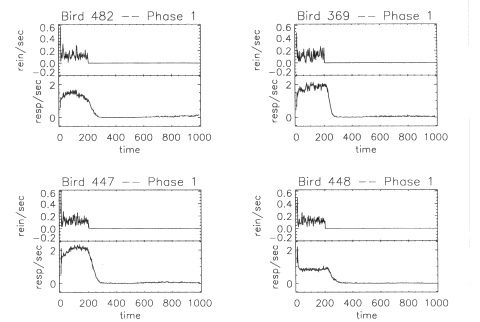
Figure 2 shows
data from 4 representative birds obtained during the steady-state
portion of Phase 1. There is considerable precision in the control of
responding during steady state by the duration of the VI schedule,
Tvi apparent in Figure 2. A similarly precise temporal control has
been shown with the peak procedure (Catania, 1970; Roberts, 1981).
The 200-s length for the VI schedule portion of the trial was
invariant and was timed irrespective of the occurrences of responding
or reinforcers, yet a noticeable change in response rate occurred
within seconds of the actual Tvi The well-defined falling edge seen
in the behavior of the 4 birds in Figure 2 is not an artifact of
averaging the steady-state trials and occurs in the data from 15 of
the 16 birds. The standard deviation of the response rate does not
noticeably increase for times close to Tvi as would have occurred if
the pigeons ceased responding over a range of times. The Phase 2
results showed similar precision in control of the behavior by the
different VI schedules and Tvi durations.

Fig. 2. Typical
repeated-trials local average reinforcement (top frame of each panel)
and supported behavior (bottom frame of each panel) for the Phase 1
step transition from a Vl schedule to extinction. The left column
shows data from the group with an exponential IRI distribution, and
the right column shows data from the group with the rectangular IRI
distribution. The scale of the scatter in reinforcement rates is
compatible with the number of reinforcers delivered during the time
used to compute the rate averages and 1/^Ncounting statistics.
The patterns of
reinforcement and response rates are not completely featureless.
There is local scatter in the reinforcement rates, which is a slight
qualitative departure from the general overview of the schedule shown
in Figure 1. Although the patterns of response rates are similar,
each bird's repeated-trials local average behavior does show some
unique characteristics.
Fourier
Transforms
The Fourier
transform is a standard mathematical technique often used as part of
an analysis of time series data (Oppenheim & Schafer, 1975). It
is particularly helpful when studying extended or intricate time
dependencies of an externally driven system. We will express the
relationship between the reinforcement schedule and the supported
behavior as a ratio of Fourier transforms. This subsection covers
Fourier transform operations in general terms as well as the specific
definition of the transform employed in this report.
A Fourier
transform decomposes a function of time into a sum of sinusoidal
(sine wave) components of different frequencies. The frequencies
required in the sum to construct a given function are determined by
the function. For example, an FI 20-s reinforcement schedule will
have a strong component at 0.05 Hz (or 1/20 s). In general, a
function that changes only slowly with time will be predominantly
composed of low frequencies; a function that changes more rapidly
will require a larger contribution from higher frequencies. The sharp
falling edge that appears in our experiment's reinforcement schedule
will require high- frequency components to be significant in the
Fourier transform. If a function of time contains structures at a
time scale of At, the Fourier transform will contain significant
components with frequencies that have half- cycle times that are at
least as short as At (i.e., f ' 1/2At). A sum of sinusoidal
components can yield nonsinusoidal shapes: Even completely
nonperiodic structures can be expressed by including the proper
sinusoidal components in the sum.
With Fourier
transforms we can isolate elements of the reinforcement schedule and
its resulting behavior that vary on different time scales. If the
behavior shows little variation over short time scales, then the
Fourier transform will be small at higher frequencies, indicating
that we can largely ignore these time scales. In addition, this
capability of Fourier transforms to separate by frequency makes
possible the solution of an integral equation, central to our
quantitative analysis, that otherwise is rather intractable.
As noted, the
basic principle of the Fourier transform is that a very broad class
of functions of time can be written as the sum of a possibly infinite
number of sine and cosine functions. An identity called Euler's
formula relates the complex exponential function with the sine and
cosine functions: e2~ifl = cos 2rrit + i sin 2rrft. Using the complex exponential, the Fourier
decomposition is expressed as a continuous summation of the form
where
H(t) could be any function of time [e.g.,
B(t)) or R(t') in Equation 3], and the function of
frequency h(f) )
is the amplitude of the
sinusoidal component contributing to the sum at frequency f In normal
usage h(f )
is simply termed the
Fourier transform of H(t)). An expression of similar form gives
h(f)) in terms of H(t):
The two members
of the H(t), h(f))
pair are just different
representations of the same information. The analytic definitions
given in Equations 1 and 2
connect this pair of time
and frequency-domain functions. Equation 1 converts a function of
frequency back to a function of time and is commonly termed the
back or inverse Fourier transform. Similarly, Equation
2 converts a function of time to a function
of frequency and is called the forward Fourier transform, or simply the Fourier
transform.
The presence of
negative frequencies in Equations 1 and 2 is a mathematical convenience. For the
present experiment, the data has only real, as opposed to complex,
values, and the Fourier transform could be defined without reference
to negative frequencies. However, such a definition uses a somewhat
nonstandard form that would raise other difficulties. The impact of
using the standard form is that the negative frequencies will simply
mirror the positive frequencies, as will be apparent in later
figures.
Although
Equations 1 and 2
are written in terms of
continuous functions of time and frequency, H(t) and h(f ), they have been implemented for discretely
sampled data (such as the 512 bin values of the repeated-trials local
averages) as a set of standard computer routines called fast Fourier
transforms (FFTs). FFT routines are efficient, well tested, and
reliable (see Press, Flannery, Teukolsky, & Vetterling, 1986, p.
381, for an extended discussion). Examples of the present
experiment's time-domain data transformed to frequency- domain data
with an FFT are given in the detailed analysis below.
The Fourier
transform is one of several types of frequency transform. All
concepts of linear analysis developed in prior work (e.g., McDowell
et al., 1993) using the Laplace transform as the link between the
time and frequency domains are the same. In fact, the Laplace
transform can be derived as a special case of the Fourier transform
(Mathews & Walker, 1965, p. 102).
Transfer
Functions and the Prediction of Behavior
The
quantitative relationship between reinforcement schedule and
supported behavior given by the transfer function holds a central
role in our efforts to predict behavior. This section covers how we
use the transfer function, first to capture the relationship of the
supported behavior to the reinforcement schedule seen in the Phase 1
data, then to predict the behavior supported in Phase 2 with a different reinforcement schedule. We
implemented the analytic expressions that define this prediction in
numerical form as part of our data- reduction software. We will work
through these computational steps using a typical bird's data to
provide a specific graphical example in the Results section below.
The c² measure for the fidelity of the
prediction is also developed in the Results section.
When expressed
as functions of time, the supported behavior at time t, B(t), and the prior reinforcement schedule,
R(t'), are related through linear analysis
(McDowell et al., 1993) by the convolution integral

The function
G(t-t') isolates the organism's contribution to the
relationship of the supported behavior to the reinforcement schedule.
In a behavioral experiment, R(t') is determined by the experimenter, and
B(t) is the measured response. Thus, if Equation 3
can be solved for G(t-t'),
it should be possible to
predict the pigeon's response to a different reinforcement schedule.
Phase 1 of this experiment is used to find the Fourier transform of
G(t - P), then Phase 2 is used to check the validity
of the resulting prediction of behavior. (It is worth noting that
R(t) and B(t) in the present work are repeated-trials
local average rates, whereas in previous work a square pulse
representation was used. Computing repeated-trials local averages for
reinforcement and response rates will yield quantities that are
equivalent to the value-like R(t) and B(t) previously used. One can assume that for
this experiment all reinforcers have a common absolute magnitude and,
similarly, all responses also have their own common absolute
magnitude. Hence, these magnitudes will not affect the computations,
and if a repeated-trials local average is computed, dividing by the
length of the time bin results in dimensions of a local average
rate.)
As discussed in
prior work (McDowell et al., 1993), the standard method to simplify
Equation 3 is by applying a frequency transform, so that Equation 3
becomes
where
b(f ), g(f ),
and r(f ) are the Fourier transforms of
B(t), G(t
— P), and
R(t'), respectively. In a relationship such as
Equation 4 that describes the transformation of an input into a
resulting output as functions of frequency, g(f ) is termed the transfer function.
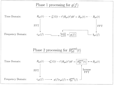
Our
data-reduction software uses Equation 4 in two somewhat different
ways to bypass Equation 3. The major processing stages for both
phases of the experiment are shown schematically in Figure 3. In each
phase, the processing yields the boxed quantity.
Fig. 3.
Schematic diagram of the steps of the data processing (see text).
Data from the first phase are used to determine the pigeon's transfer
function, g(f) Data from the second phase are used to predict the
pigeon's behavior BPr2'd(t) and the prediction is compared to the
measured behavior Bp2(t). FFT routines provide the needed
transformations between the time domain and the frequency domain and
are shown as the vertical arrows labeled FFT and Inverse FFT.
Data from the
first phase determine the transfer function, g(f ), for a specific subject. The three steps in
the Phase 1 (pi) processing are:
1. Transform
the measured reinforcement rate as a function of time,
Rpl (t), to the function of frequency, rpl (f
).
2. Transform
the measured response rate as a function of time, Bp~(t), to the function of frequency,
bp~ (f ).
3. From
Equation 4, compute the transfer function as a function of frequency,
g(f ), by division:
If a linear
analysis is appropriate for simple schedule behavior, then the
transfer function should isolate the characteristics of the specific
organism under study and should not depend on the particular
reinforcement input and response output used in its determination.
The Phase 2 (p2) processing uses this assumed independence to predict
the responding that ought to be seen with a new reinforcement
schedule. There are again three steps in the processing:
1. Transform
the measured reinforcement rate as a function of time, Rp2(t), to the
function of frequency, rp2(f).
2. Compute the
predicted Phase 2 responding, bpr2ed (f ), as a function of frequency using the
transfer function, g(f ),
obtained in Phase 1. The
prediction is given by Equation 4:
3. Inverse
transform the predicted response rate as a function of frequency,
bpr~ed(f) to a function of time, Bp2ed(t), for comparison to the
response rate actually measured, Bp2 ( t) .
It is important
to note that Bpr~ed(t) is an absolute prediction based solely on the
Phase 1 measurement of g(f
) and the Phase 2
reinforcement schedule, Rp2(t); no free (or adjustable) parameters
are used in the prediction (beyond the determination of
g(f) in Phase 1).
There are
technical points germane to our FFT-based data reduction that are,
for the most part, more of interest to students of numerical analysis
than of behavior analysis, so we simply note their existence here.
They are dealt with in the Appendix, which presents a tutorial test
case of linear analysis that is appropriate to the data-reduction
problem at hand. Their chief effect is to produce spike artifacts in
transfer functions computed with Equation 5. In general, the effects
of these artifacts will not be important in the prediction of
behavior because they occur mainly at higher frequencies and have
random phases. The important point for the reader to keep in mind is
that although our data-reduction method is a sound means of
extracting transfer functions, care is required in its actual use.
RESULTS
Bird 369:
Step-by-Step Analysis and Intermediate Results
This subsection
illustrates the data-reduction processing stages and displays the
important intermediate results graphically for 1 of the 16 birds in
this study. Bird 369 was selected as an example solely because it had
the lowest serial number. With the exception of Bird 451 noted below,
the data from any bird could have been used to illustrate the
analysis. As discussed above and shown in Figure 3, the processing
stages use Phase 1 reinforcement and response data to extract a
transfer function and then make a prediction of the Phase 2
responding.
The data
reduction begins with collecting the reinforcement and response times
from all trials after stability and computing the repeated-trials
local averages for reinforcement and response rates. The
reinforcement rate as a function of time, Rpl(t), for Bird 369 is
shown in the top frame of the upper right panel of Figure 2. The
response rate as a function of time, Bpl (t), for Bird 369 is shown in the lower frame of
the same panel of Figure 2. Note that the scatter or noise in
Bp,(t) is relatively smaller than the scatter in
Rp~(t). Also note that the sharp edge in
Rpl ( t) at the onset of extinction produces a
softer falling edge in the bird's behavior seen in Bpl(t).
The data from
the experiment are discrete sets of rate samples over a finite time
interval. This finite sampling resolution in the time domain is
reflected in a corresponding finite sampling resolution in the
frequency domain. The frequency scale produced by an FFT routine
follows from the sampling rate employed. In this experiment, the
trial length, Ttrial limits the lowest frequency component to
or 1 mHz (1 mHz
= 0.001 Hz) for the 1,000s trials used. The highest frequency
component is set by the Nyquist critical frequency, given by
where
D
is the time period between successive samples. Because the rates are
computed for 512 time bins over the 1,000-s trials, the highest
frequency components are at ±256 mHz.
These two limits mean that in the frequency domain we can determine
r(f), b(f), and g(f) at frequencies of -255 mHz, - 254 mHz, . . .. -1
mHz, 0 mHz, + 1 mHz, + 2 mHz, . . .. +255 mHz, +256 mHz. For further
explanation of FFT routine frequency scales and Equations 7 and 8,
please refer to Press et al. (1986).
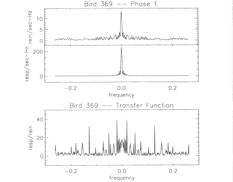
The amplitude
of the reinforcement rate as a function of frequency, |rpl(f)l, for
Bird 369 is shown in the top panel of Figure 4. Because |rpl(f)l is
an amplitude per unit frequency range, the units are reinforcers per
second Hertz (or reinforcers per second divided by Hertz). A
frequency-domain phase plot also exists because rpl(f) is a complex
function. The phase information is essential if one is actually doing
the computations with Equation 5. For the discussion in this paper,
however, the amplitude plots are sufficient. The form of |rp(f)| is
typical of an FF 1 for experimental data. The lower frequencies
contain most of the meaningful structure of the data and the higher
frequencies have approximately equal amplitudes per frequency bin. To
have equal amplitudes per frequency bin is characteristic of white
noise; this region is termed the noise floor and is considered not to contain useful
information. The low-frequency boundary of the noise floor for
|rp(f)| is not sharply defined, but begins no later than +100 mHz.
The amplitude of the response rate as a function of frequency
|bpl(f)l, for Bird 369 is shown in the middle panel of Figure 4.
Comparing Bird 369's time-domain plots of Figure 2 and frequency
domain plots in Figure 4, one can see that the sharp edge at 200 s
and the fast fluctuations in the reinforcement rate Rpl(t) generate
substantially greater amplitudes at higher frequencies' in |rpl(f)l
than are generated in lbp (f ) | by the softer (slower) falling edge
and steadier response rate of Bp(t).

Fig. 4. The
Phase I results for Bird 369 displayed in the frequency domain and
the amplitude of the resulting transfer function (see text). Note the
expected symmetry about zero is apparent in r(f), b(f),), and g(f)
By comparing
the frequency-domain amplitude plots for Bird 369's reinforcement and
response rates in Figure 4, one can see graphically the basic
character of the transfer function. The behavior of Bird 369 is
affected primarily by the low frequencies, rather than the higher
frequencies, that are present in the input reinforcement. In the
language of linear analysis, one would describe Bird 369 as operating
as a form of low- pass filter.2 Furthermore, all birds in this
experiment have transfer functions with this same general lowpass
character. These transfer functions allow prediction of the Phase 2
responding, in part, by quantifying how much each bird will filter
out the higher frequencies.
The amplitude
of the transfer function as a function of frequency, |g(f)|, for Bird
369 is shown in the bottom panel of Figure 4. For low frequencies,
roughly f '
30 mHz, the transfer
function is substantially larger than unity. These low- frequency
values of the transfer function reflect that the pigeon's overall
response rate (typically 2.5 responses per second) is faster than the
reinforcement rate (typically 1 reinforcer per 20 s). The relative
size of the transfer function at low frequencies compared to higher
frequencies means that the resulting behavior is primarily a function
of the longer time scales in the reinforcement schedule, such as the
transition from VI to extinction that occurred once per 1,000 s.
There are, however, many spikes in the higher frequency region. From
Figure 4 one can see that these spikes occur mostly at frequencies
for which both the reinforcement input and the response output
amplitudes are determined mainly by noise. These spikes are generated
at frequencies where rpl(f) is very small. The spikes will not
greatly affect the prediction made with Equation 6, Because at these
higher frequencies, rp2(f) will also be small. Still, one direction
for future work will be reducing these effects of measurement noise
on the computations.
With the
measurement of the transfer function, g(f), in hand, we can now predict the behavior
that will be supported in steady state by a new schedule. We assigned
Bird 369 to the Phase 2 test schedule group that had the same VI 20-s
schedule and changed the step transition time, Tvi to 300 s. The
experimentally measured repeated-trials local average response rate
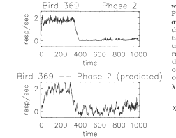
as a function of time, Bp2(t), for Bird 369 during Phase 2 is shown
in the top panel of Figure 5. The predicted response rate as a
function of time during Phase 2 Bp2ed(t), found using the transfer
function of Figure 4, is shown in the bottom panel of Figure 5. On
the whole, the predicted behavior agrees with the measured behavior.
(A c² assessment of that agreement is
presented below.)
Fig. 5. The
experimentally measured response rate as a function of time, Bp2(t),
for Bird 369 during Phase 2 is shown the top panel. The predicted
response rate, BPpy'd(t), for Bird 369 during Phase 2 is shown in the
bottom panel.
The computation
of the transfer function and prediction is the very simplest one
could do. This prediction was made using Ttrial = 1,000 s, which
ignores the difficulties caused by the commensurate frequencies of
zero amplitude discussed in the Appendix. No effort was made to
reduce the effects of noise. In addition, there are time periods
during which the bird is predicted to have an unattainable negative
response rate. Iterative methods do exist to constrain the transfer
function, so responding is always greater than or equal to zero, but
the implementation of such constraints would take us far afield.
c²v Measure and Overall Results
We predicted
the Phase 2 behavior for the remaining 15 birds with the same
data-reduction routines we used on Bird 369's data. We also predicted
the behavior for all 16 birds with the common time base length,
Ttrial changed from 1,000 s to 977.11 s (the rationale for the second
value of Ttrial is given in the Appendix). Currently, no other
analyses make predictions for the detailed steady-state form of
B(t). Hence, we are limited in quantitative
evaluation of the results to measuring the discrepancy from a perfect
prediction, that is, the discrepancy from the real observed Phase 2
data.
As a global
measure of our Phase 2 predictions' accuracy, we used c²v, the
reduced c² of the discrepancy between Bp2ed(t),
the linear system prediction, and Bp2 ( t), the pigeon's measured responding. The
expression for c²v is given in this case by
(Bevington, 1969, p. 187)
where ~2 is the
variance in the ith measured Phase 2 response rate, Bp., ( tj) .
Estimating ~Bp2 j during extinction is problematic because the
response rate is so low that some of the time intervals contain no
responses for any trial, leading to Bp2(t;) - 0 and a2B2j0. A reasonable estimate of the variance
during the extinction interval is O.Bp2FXT, the average of those
actually measured (including those of zero value). Thus the
expression used for c²v becomes
where tm is the
time closest to the onset of extinction at Tvi. Note that the
normalizing factor that appears in Equation 10 is 1/N because there
are no free parameters in Bp2ed(t). Hence, the number of degrees of
freedom is equal to the number of data points.
The values of
c²v for all birds in this study are
shown in Table 1 computed both with Ttrial at the full 1,000 s and at
977.11 s. Because both Equations 9 and 10 are measures of a
prediction's discrepancy, the lower the value of c²v, the
better the quality of the prediction. The c²v values
specify the probability that a random (or chance) prediction could be
as close to the data as our prediction. The distribution of
c²v values was noticeably bimodal. In
the majority of cases, agreement between the actual Phase 2
responding and our prediction is better than chance for a p < .01
threshold. (For N == 512, the agreement between the predicted and
obtained behavior occurs by chance less than one time in 100 when the
c²v is less than 0.8603.) When the
prediction failed, the values of c²v were at
the other extreme. (The agreement between the predicted and obtained
behavior occurs by chance at least 99 times in 100 when the
c²v is greater than 1.1511. )
Table 1
The values
of c²v for the birds in this study.
|
Bird
|
x~2 (1,000
s)
|
c² (977.11 s)
|
|
|
|
Phase I Fleshler-Hoffman:
VI 20, Tvi = 200 s
|
|
Phase 2 Fleshler-Hoffman:
V1 40, Tvi = 300 s
|
|
424
|
0.4791
|
0.5601
|
|
467
|
0.3615
|
0.4892
|
|
468
|
1.1792
|
1.3879
|
|
482
|
0.4280
|
0.4865
|
|
|
|
Phase 1 Fleshler-Hoffman:
V1 20, Tvi = 200 s
|
|
Phase 2 Fleshler-Hoffman:
V1 40, Tvi = 200 s
|
|
447
|
0.6110
|
0.2627
|
|
460
|
0.2779
|
0.4455
|
|
461
|
1.0350
|
0.9656
|
|
475
|
0.2794
|
0.2826
|
|
|
|
Phase 1 rectangular: VI
20, Tvi = 200 s
|
|
Phase 2 rectangular: VI
20, Tvi = 300 s
|
|
369
|
0.5880
|
1.3112
|
|
438
|
10.1653
|
2.1843
|
|
445
|
1.4199
|
0.5767
|
|
451
|
1.0879
|
0.9083
|
|
|
|
Phase 1 rectangular: VI
20, Tvi = 200 s
|
|
Phase 2 rectangular: VI
40, Tvi = 200 s
|
|
426
|
0.4322
|
0.9747
|
|
448
|
1.5433
|
2.4711
|
|
454
|
0.3737
|
0.3904
|
|
488
|
3.3400
|
3.5335
|
Note. Tvi
indicates the length of
time during the trial that the Vl schedule was in effect.
The reader
should be mindful that Equation 10 measures the overall quality of
the prediction. There are smaller features in most birds' Phase 2
responding that are not accurately predicted. Even so, the fidelity
to observed detail in the measured behavior by predicted behavior can
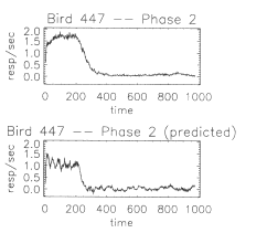
be reasonably good. As an example, Figure 6 shows the measured and
predicted Phase 2 responding of Bird 447. Also note that a bird's
transfer function is unique to that specific bird. For example, the
best Phase 2 prediction (lowest c²) for
Bird 369 is made with Bird 369's own transfer function.
Fig. 6. The
experimentally measured response rate as a function of time, Bp2(t),
for Bird 447 during Phase 2 is shown the top panel. Note that the
data set has been truncated slightly so Ttrial = 977.11 s (see
Appendix). The predicted response rate, BpPed ( t), for Bird 447 during Phase 2 is shown in the
bottom panel.
In most cases
in which the prediction was unsatisfactory, the difficulties could be
traced to a processing artifact that occurs in Equation 5. As has
been noted and is discussed further in the Appendix, at some
frequencies the amplitude of Rpl, (f) can be quite small and can
result in a narrow spike in the transfer function. The data from Bird
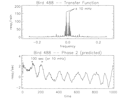
488 provide a good illustration of the artifact and its effect on the
prediction. The top panel of Figure 7 shows the amplitude of the
transfer function. Note the large spikes at +10 mHz. The bottom panel
of Figure 7 shows the predicted Phase 2 behavior. A large 10-mHz
oscillation is clearly apparent in the prediction. However, if we
remove the most serious spike artifacts by replacing the values g(f)
with nearest neighbor averages at the +10-mHz and +5mHz spikes, we
reduce the discrepancy between the predicted and the obtained
behavior. The revised prediction had a c² of
1.2023, improved by roughly a factor of three. There are more formal
and mathematically rigorous methods to correct for such spike
artifacts, but clearly the entire problem can be simply avoided. In
future experiments, the schedule of reinforcement used in the
measurement of the transfer function should be selected so that the
amplitude of rpl(f) is significantly greater than zero in the
frequency region of interest.

Fig. 7. The
amplitude of the transfer function, |g(f)|, for Bird 488 is shown the
top panel. The predicted response rate, Bp2(t), for Bird 488 during
Phase 2 is shown in the bottom panel.
The response
pattern of one of the birds, Bird 451, was unique and caused the data
reduction and prediction methods to fail in an interesting manner.
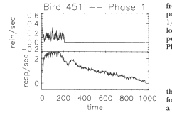
The Phase 1 reinforcement and responding are shown in Figure 8.
Unlike all other birds in this study, Bird 451 responded at a
relatively high rate throughout Ttrial (including the entire 800-s
extinction period). This violates a restriction of our FFT-based
computation. Recall from Equation 7 that the lowest nonzero frequency
component that the FFT will determine is for the frequency 1/ Ttrial
In the case of Bird 451, the behavior in the time domain would have
continued during extinction for a longer time than the limit imposed
by Ttrial Hence, in the frequency domain there are behaviorally
important frequency components below the 1/Ttrial limit. Because the
FFT excludes these lower frequencies from the computations, the
prediction does not agree with the measured Phase 2 behavior to any
significant extent.

Fig. 8. The
experimentally measured reinforcement rate as a function of time,
Rpl(t), for Bird 451 during Phase I is shown in the top panel. The
measured response rate, Bpl.(t), for Bird 451 during Phase I is shown
in the bottom panel. Compare this bird's response pattern to those of
Bird 369 (Figures 2 or 5), Bird 447 (Figure 6), or any of the other
birds shown in Figure 2.
DISCUSSION
The conclusions
that can be drawn from this study are that (a) the general
qualitative form for pigeons' transfer functions is that of a
low-pass filter, and ((b)) using the experimentally measured transfer
function allows some predictability of the pigeons' behavior under a
different set of contingencies. The present experiment is the first
effort to extract a transfer function from experimental data and the
first to use a linear analysis to predict behavior dynamics, albeit
in a repeated-trials local average steady state. The values of XY are
reasonably good for a prediction without free parameters, suggesting
at least some measure of confidence in the application of linear
analysis to behavior. Whether other methods, linear or not, can make
comparable or superior predictions of future dynamic behavior based
on prior experimental observations remains an open question.
A variety of
past work has sought to characterize a reductionistic process that
could result in the functional properties obtained between temporal
requirements and obtained behavior. These efforts are exemplified by
a number of models based on internal pacemakers (Church, 1984;
Gibbon, 1991; Killeen, 1991). In contrast, the transfer function
provides a quantitative method to capture an external view of the
empirical relationship between the temporal properties of
environmental contingencies and the supported behavior. Consequently,
our analysis is silent on an internal view and does not distinguish
or contradict the various timing models. However, should one of these
models of timing be recast for application to our experimental
procedure, a prediction of low-pass behavior must fall out naturally.
In addition, our experiment is silent on the mechanism that causes
short IRI distributions to be preferred. The low-pass character
applies to the overall dynamic structure of the trial.
Based on the
results of this experiment, one can now refine the measurement of a
steady-state transfer function, and more demanding tests can be
designed. From the standpoint of linear analysis, this experiment's
results, particularly the low-pass character of the transfer function
and the existence of computational spike artifacts, provide important
guideposts for improvement. In future work, the reinforcement
schedule should permit more detailed study of the lower frequency
domain (i.e., frequencies of roughly +150 mHz). The reinforcement
schedule will also have to be carefully chosen to prevent the
occurrence of zero or near-zero amplitudes within this behaviorally
significant frequency domain.
REFERENCES
Anderson, L.
W., & Beeman, W. W. (1973). Electric circuits and modern electronics
(pp. 137-138). New York:
Holt, Rinehart and Winston.
Baum, W. M.
(1979), Matching, undermatching, and overmatching in studies of
choice. Journal of the
Experimental Analysis of Behavior, 32, 269-281.
Bevington, P.
R. (1969). Data reduction
and error analysis for the physical sciences. New York: McGraw-Hill.
Catania, A. C.
(1970). Reinforcement schedules and psychophysical judgments: A study
of some temporal properties of behavior. In W. N. Schoenfeld (Ed.),
The theory of reinforcement
schedules (pp. 1-42). New
York: Appleton-Century-Crofts.
Church, R. M.
(1984). Properties of the internal clock. In J. Gibbon & L. Allen
(Eds.), Timing and time
perception (pp. 566-582).
New York: New York Academy of Sciences.
Fleshler, M.,
& Hoffman, H. S. (1962). A progression for generating
variable-interval schedules. Journal of the Experimental Analysis of
Behavior, 5, 529-530.
Galbicka, G.
(in press). Rate and the analysis of behavior: Time to move forward?
In L. J. Hayes & P. M. Ghezzi (Eds.), Investigations in behavioral epistemology.
Reno, NV: Context Press.
Galbicka, G.,
Kautz, M. A., & Jagers, T. (1993). Response acquisition under
targeted percentile schedules: A continuing quandary for molar models
of operant behavior. Journal of the Experimental Analysis of
Behavior, 60, 171-184.
Gibbon, J.
(1991). Origins of scalar timing. Learning and Motivation, 22,
3-38.
Killeen, P. R.
(1991). Behavior's time. In G. H. Bower (Eds.), The psychology of learning and motivation
(pp. 295-334). New York:
Academic Press.
Mathews, J.,
& Walker, R. L. (1965). Mathematical methods of physics.
New York: W. A. Benjamin.
McDowell, J.
J., Bass, R., & Kessel, R. (1992). Applying linear systems
analysis to dynamic behavior. Journal of the Experimental Analysis of
Behavior, 57, 377-391.
McDowell, J.
J., Bass, R., & Kessel, R. (1993). A new understanding of the
foundation of linear system theory and an extension to nonlinear
cases. Psychological
Review, 100, 407-419.
Oppenheim, A.
V., & Schafer, R. W. (1975). Digital signal processing. Englewood Cliffs, NJ: Prentice Hall.
Palya, W. L.,
& Walter, D. E. (1993). A powerful, inexpensive experiment
controller or IBM PC interface and experiment control language.
Behavior Research Methods,
Instruments, & Computers, 25, 127-136.
Press, W. H.,
Flannery, B. R., Teukolsky, S. A., & Vetterling, W. T. (1986).
Numerical recipes the art
of scientific computing. Cambridge: Cambridge University Press.
Roberts, S.
(1981). Isolation of an internal clock. Journal of Experimental Psychology: Animal Behavior
Processes, 7, 242-268.
APPENDIX
Computation of
a transfer function by dividing two FFTs, as is done by Equation 5,
does introduce some artifacts into the data processing. Such
difficulties with divisions are fairly standard in frequency-domain
work, because many time-domain functions yield frequency-domain
functions with zero amplitude for some particular frequencies and/or
for all frequencies higher than some cut-off frequency. Thus,
r(f) can easily be zero (or very close to it)
for a range of frequencies, and Equation 5 cannot be evaluated within
this range. For an ideal linear system, b(f) would also be zero at these frequencies and
result in the indeterminate expression of 0/0 for g(f ). This problem is exacerbated by the fact
that computer FFT algorithms do not perform true Fourier transforms
over a continuum of frequencies, but instead perform a discrete
Fourier transform (FFT): an approximation using a discrete set of
frequencies (Oppenheim & Schafer, 1975; Press et al., 1986). As
will be shown below, the sharp step from a static VI schedule to a
period of extinction in the time domain can produce a discrete set of
frequencies at which r(f )
= 0.
A test case
will illustrate the use of FFT based routines to solve a linear
analysis problem and provide some insight into the technique's
stability and limitations. Unlike the behavior of a pigeon, we have
an excellent theoretical model for the behavior of the electrical
circuit used as the test case. As a result, we are able to compare
the transfer function found by division of output by input with the
correct transfer function. We shall see how the problems, primarily
noise and zero-amplitude frequencies, introduce spike artifacts into
the computed transfer function. We should expect the same effects to
appear in any real data of similar form.
This test case
is a standard low-pass electrical filter normally built with a
resistor and capacitor in series and commonly referred to as an
RC low-pass f filter
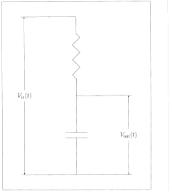
The circuit is shown in
Figure 9. Extended discussion of this circuit can be found in most
basic electrical circuits textbooks (e.g., Anderson & Beeman,
1973, p. 137). The most important point about this circuit for the
present discussion is that it is completely linear. This means that
an expression of Equation 3's form relates the output voltage to the
input voltage:
In the
frequency domain the voltages are related by
Beyond
satisfying the general relations of Equations 11 and 12, an RC
low-pass filter is a convenient test case because closed-form
analytic expressions exist for both gRc(f) and a Vin (
t), Vout ( t)
pair.
Fig. 9. A
resistor-capacitor (RC) low-pass filter. The characteristic time
constant of such a filter is given by T = RC Vin(t) and Vout(t) indicate the input and
output voltages as functions of time.
Commensurate
Frequencies of Zero Amplitude
We will begin
with a Vn(t), Vout(t) pair that is reasonably similar to the
R(t), B(t) pairs observed in the actual data of this
study.
We choose the
input voltage shown in the top panel of Figure 10. The analytic
expression for a square step in the time domain is
The output
voltage generated by an RC lowpass filter in response to the input
square step given by Equation 13 is
and is shown in
the bottom panel of Figure 10.
Fig. 10. A
square step input voltage (Vin) is shown in the top panel. The bottom
panel shows the output voltage (Vout) from the circuit shown in
Figure 9.
The analytic
expression for the transfer function of an RC low-pass filter is
where the phase
angle is
and the
filter's critical frequency, fo, is a characteristic of the filter
related to its time constant, T = RC, by
The transfer
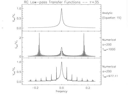
function's amplitude, |gRC(f)l, computed with Equation 15, is shown
in the top panel of Figure 11.
Fig. 11. The
top panel shows the transfer function of an RC low-pass filter as
computed directly from the circuit's electrical properties. The
middle panel shows the transfer function computed with discretely
sampled values from Equations 13 and 14, where a = 200 and Ttrial =
1,000. The bottom panel shows the transfer function computed with
discretely sampled values from Equations 13 and 14, but where a = 200
and Ttrial = 977.11.
Equations 13
and 14 provide an input-output pair in the correct form to run
through the Phase 1 processing described in the text and shown
schematically in Figure 3. Accordingly, the middle panel of Figure 11
shows the |gRC(f)| that results when the Vin(t, Vout(t) pair shown in
Figure 10, which has a = 200, Ttrial = 1,000, and t = 35, is run
through the data-reduction software. The disagreement between the
actual and computed RC lowpass transfer functions is apparent and
illustrative of the problems encountered in reducing the data from
our experiment. When Equation 13 is transformed into the frequency
domain with Equation 2, one obtains

Note that for
nonzero frequencies, the factor sin (2qrfa/2) will cause v,n(f) to be zero if fa is an
integer. If a = 200 and Ttrial = 1,000, fa is exactly an integer at f
= +5 mHz, +10 mHz, +15 mHz, . . ., and so forth. Note that the
Fourier transform of Vout(t)' is, from Equation 12, also zero at
these frequencies. The significance to our data reduction is that, in
an unanticipated mathematical coincidence (caused by selecting a
value of Tvi that is a simple rational fraction of Ttrial, e.g., 1/5
for Phase 1), these same frequencies are used, because of the
discrete Fourier transform, to evaluate Equation 5. This accounts for
the large artifacts at every fifth frequency shown in the middle
panel of Figure 11. At the remaining frequencies, the transfer
function values computed by the data-reduction software agree, within
machine precision, to the correct values calculated directly with
Equation 15.
As a simple
refinement to the data reduction that avoids this problem of
commensurate frequencies of zero amplitude, we can exclude a small
interval from the end of the trial. This introduces a slight offset
between all the FFT component frequencies defined by Equation 7 and
the zeros of Equation 18. To generate this offset, we arbitrarily
chose Ttrial = 977.11 s and ignored the data from the last 22.89 s of
each 1,000-s trial. The bottom panel of Figure 11 shows the IgRC(f)I
that results for a Vin(t), Vout(t) pair that has a = 200, Ttrial =
977.11, and t = 35. The change in the FFT routine
frequency scale obtained by changing Ttrial is small, 2.3% in f1, but
it is sufficient to avoid the zero-amplitude frequencies when fa is
an integer. As a result, the transfer function computed from this
Vin(t), Vout(t) pair agrees closely with the correct transfer
function shown in the top panel. However, there are still some
frequencies that, although not exactly commensurate with a
zero-amplitude frequency, are quite close to these frequencies. At
such frequencies, which occur roughly every 45 mHz, the transfer
function is improperly determined.
Impact of
Noise
Across a broad
band of the higher frequencies measured in this experiment, the
amplitudes of both r(f )
and b(f ) are small and are dominated by random
noise. The noise has the minor advantage that the actual occurrence
of a zero denominator (discussed above) almost never happens, but,
obviously, the computed g(f) ) will not be reliable when either the
numerator or denominator in Equation 5 is dominated by noise. The
ultimate effect is that the predicted Phase 2 responding will always
be noisier than the actual data.
One can
accurately simulate experimental data that contain noise (rapid
uncorrelated fluctuations) and use the RC low-pass filter test case
to study how noise limits the method's resolution. The overall result
of these tests is that the resolution of our data-reduction method
decreases as the noise increases.
Figure 12 shows
a Vin(t), Vout(t) pair to which we have added a moderate amount of
Gaussian-distributed random noise. To mimic the experiment's
reinforcement data, the Vin(t) shown in Figure 12 has no added noise
during the period corresponding to extinction in the actual
experiment. We found, somewhat counterintuitively, that removing the
noise from this portion of the input increases the data- reduction
software's sensitivity to noise.
Fig. 12. The
top panel shows an input to an RC lowpass filter with Gaussian noise
added. The bottom panel shows an output from an RC low-pass filter
with Gaussian noise added.
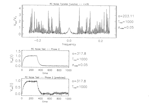
Figure 13 shows
the results generated by our data-reduction software when the Vin(t),
Vout(t) pair from Figure 12 is used to compute a transfer function,
gRC noise(f)) The top panel shows the amplitude of the transfer
function IgRC,noise(f)l. Although the low-frequency values of the
transfer function are faithful to IgRC(f)l, for frequencies beyond
+50 mHz the noise causes large spikes in the transfer function. As
one increases the noise amplitude, these spikes appear at lower
frequencies. The middle panel shows an output voltage computed
directly from the circuit's electrical properties when the input step
lasts for 317.8 s instead of 203.11 s with a noise addition:
Vout,noise(t). The bottom panel shows the predicted output voltage,
VOuetdnoise(t), computed with the derived transfer function,
gR,.noise(f).

Fig. 13.
Results generated by our data-reduction software when the Vin(t),
Vout(t) pair from Figure 12 is used. The top panel shows the
amplitude of the transfer function as a function of frequency,
|gRC,noise(f)|. The middle panel is an output voltage computed
directly from the circuit's electrical properties with an appropriate
noise envelope Vout,noise(t) The bottom panel shows predicted output
voltage as a function of time, Vjnrr~dn,,j=(t), computed with the
derived transfer function. Note that the bottom two panels of this
figure are functions of time, whereas the top panel is a function of
frequency.
Because both
Vin(t) and Vout(t) have noise, it should not be surprising that the
prediction will have more noise than either one. The division in
Equation 5 will increase the relative noise amplitude on average by a
factor of about N/2 for the lower frequencies when noise is not, in
general, a substantial problem. At higher frequencies when the
noisefree amplitudes for vin(f) and vout(f) are small, the noise
contribution to |gRC,noise(f) Will dominate. A possible refinement of
the data reduction would be smoothing of these high frequency spikes.
Finally, during the evaluation of Equation 6, a second increase in
relative noise amplitude will occur.
Footnotes
1 The amplitude
of |rp(f)| is larger relative to the size of the zero frequency
component spike than the amplitude of |bp1(f)| at most frequencies.
2 There are
many other types of low-pass filters beyond the simple
resistor-capacitor low-pass filter discussed in the Appendix.
Authors'
Notes
The authors
gratefully acknowledge the contribution of Helen Bush and Josey Chu
for meticulously running the birds; Elizabeth Palya for contribution
in all phases of this research; and Bo Codella, Greg Galbicka, and
Bernard Hill for their helpful comments and suggestions on earlier
drafts of this paper. Portions of this paper were presented at the
Society for the Quantitative Analysis of Behavior, May 1994.
The addresses
for questions and other correspondence are Bill Palya or Don Walter,
Department of Psychology, Jacksonville State University,
Jacksonville, Alabama 36265. Bob Kessel is now at Naval Center for Space
Technology, Code 8001.1, Naval Research Laboratory, Washington, D.
C.. 20375-5354. Bob Lucke is now at Remote
Sensing Physics Branch, Code 7220, Naval Research Laboratory,
Washington, D. C.. 20375-5352. The data
reduction software used for the linear analysis based prediction is
available from JSU program archive. The raw data logs are also
available upon request from the JSU data archive.
Received
August 2, 1995
Final
acceptance July 24, 1996


Date Last Reviewed : May 26, 2003


