Disclaimer
This information has the status of "out-takes." There is no reason to believe that any of it is wrong, but it hasn't been checked, double checked, then checked again. They are the data, analyses, or figures which were not published and it seems a waste to simply delete the files. The data are provided in the event someone can benefit by the additional information. They are not intended for the casual pursuer and presume a prior reading of the JEAB paper and a cooperative mind set.
If you note a discrepancy between this information and the published version of the research, the published version is very probably correct. If you'd like further information or a further explanation of any of the material or, if something appears discrepant, let me know. Unless this web appendix received sufficient traffic, I just can't justify the time necessary to provide the information in a more immediately digestible form - sorry.
Our experiments are carried out by computer programs. A nomenclature is used to specify the program. All programs start with E. The subsequent digits are the experiment number (e.g., E43) the following letters are the procedure "phase" (e.g., E43C). The digits following that indicate the variant of the procedure such as counterbalancing color or using the two outside keys versus using adjacent keys (e.g., E43C1).
The following procedures were carried out.
E43
Group 1 Training Phases (CONCURRENT VI xx VI xx)
Group 2 Training Phases (CONCURRENT VI xx VI xx)
| |||||||||||||||||||||||||||||||||||||||||||||||||||||||||||||||||||||||||||||||||||||||||||||||||||||||||||||||||||||||||||||||||||||||||||||||||||||||||||||||||||||||||||||||||||||||||||||||||||||||||||||||||||||||||||||||||||||||||||
NOTE!
The internal phase numbers are not the same as those appearing in JEAB, and a number of procedures were carried out which do not appear in JEAB.
5-min trial
15-sec blackout between trials
| Phase | Sess | Condition Name | Dates Run |
| 5 | 60-65 | E43C1/2 COD 1.5 s | 9/10/97 - 11/29/97 |
| Group 1: E43C1 VI 15-sec -->VI 480-sec on KL turquoise VI 480-sec-->VI 15-sec on KR orange | |||
| JEAB Phase 1 | Group 2: E43C2 VI 480-sec -->VI 15-sec on KL turquoise VI 15-sec -->VI 480-sec on KC orange | ||
| 6 | 60 | E43D1/2 (key reversal) COD 1.5 s | 11/30/97 - 1/31/98 |
| Group 1: E43D1 VI 480-sec --> VI 15-sec on KL turquoise VI 15-sec --> VI 480-sec on KR orange | |||
| JEAB Phase 2 | Group 2: E43D2 VI 15-sec --> VI 480-sec on KL turquoise VI 480-sec --> VI 15-sec on KC orange | ||
| 7 | 60 | E43E1/2 - Clock added COD 1.5 s | 2/1/98 - 4/1/98 |
| Group 1: E43E1 VI 480-sec --> VI 15-sec on KL clock VI 15-sec --> VI 480-sec on KR clock | |||
| Group 2: E43E2 VI 15-sec --> VI 480-sec on KL clock VI 480-sec --> VI 15-sec on KC clock | |||
| 8 | 100 | E43F1/2 - Hue order clock COD 1.5 s | 4/2/98 - 7/11/98 |
| Group 1: E43F1 VI 480-sec -->VI 15-sec on KL hue clock VI 15-sec -->VI 480-sec on KR hue clock | |||
| JEAB Phase 3 | Group 2: E43F2 VI 15-sec --> VI 480-sec on KL hue clock VI 480-sec --> VI 15-sec on KC hue clock | ||
| 9 | 80 | E43G1/2 - Hue order clock COD 1.5 s | 7/12/98 - 9/29/98 |
| Group 1: E43G1 VI 15-sec --> VI 480-sec on KL hue clock VI 240-sec on KR hue clock | |||
| Group 2: E43G2 VI 15-sec --> VI 480-sec on KL hue clock VI 240-sec on KC hue clock | |||
| 10 | 90 | E43H1/2 COD 2.5 sec | 9/30/98 - 12/29/98 |
| Group 1: E43H1 | |||
| Group 2: E43H2 | |||
| 11 | 90 | E43I1/2 COD 2.5 sec | 12/30/98 - 4/3/99 |
| Group 1: E43I1 VI 15-sec --> VI 480-sec on KL orange VI 240-sec on KR turquoise | |||
| Group 2: E43I2 VI 15-sec --> VI 480-sec on KL orange VI 240-sec on KC turquoise | |||
| 12 | NOTE: No phase 12 - it was skipped in database by mistake. It was too much trouble to fix the error. | ||
| 13 | 115 | E43C1/2 (same as Ph 5) | 4/4/99 - 8/3/99 |
| Group 1: E43C1 | |||
| JEAB Phase 4 | Group 2: E43C2 | ||
| On hold | 8/4/99 to 2/5/00 | ||
| 14 | 35 | E43J1/2 COD 1.5 sec VI 50-sec with probabilistic allocation of reinforcement | 2/6/00 - 3/12/00 |
| Group 1: E43J1 KL turquoise --> p (1.0 to .01) KR orange --> p (.01 to 1.0) | |||
| Group 2: E43J2 KL turquoise --> p (.01 to 1.0) KC orange --> p (1.0 to .01) | |||
| 15 | 90 | E43K1/2 (same as Ph 14 except NO COD) | 3/13/00 - 6/10/00 |
| JEAB Phase 5 | |||
| On hold | 6/11/00 to 7/7/01 | ||
| 16 | 46 | E43K1/2 (same as Ph 15) | 7/8/01 - 8/22/01 |
| JEAB Phase 5 | |||
| On hold | 8/23/01 to 10/12/01 | ||
| 17 | 50 | E43L1/2 COD 1.5 sec | 10/13/01 - 12/05/01 |
| Group 1: E43L1 KL turquoise --> p (.067to .002) KR orange --> p (.002 to .067) | |||
| JEAB Phase 6 | Group 2: E43L2 KL turquoise --> p (.002 to .067) KC orange --> p (.067 to .002) | ||
| 18 | 50 | E43M1/2 COD 1.5 sec | 12/6/01 - 1/24/02 |
| Group 1: E43M1 KL turquoise --> p ((.002 to .067) KR orange --> p (.067 to .002) | |||
| JEAB Phase 7 | Group 2: E43M2 KL turquoise --> p (.067 to .002) KC orange --> p (.002 to .067) | ||
ABA Presentation Slide Set
(Palya & Powell, ABA 2000)
A good, imaged-based introduction to the rationale underlying the research and an overview of the procedures, data, analysis, and results.
ABA 2000 Slide Set
 Slide 1
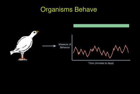 Slide 2
Organisms behave, a live animal is not the same as a dead animal.
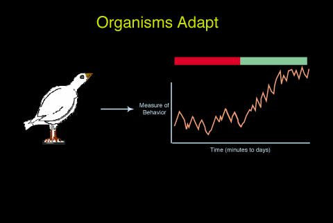 Slide 3
Not only do animals behave, they "learn" - they benefit from experience.
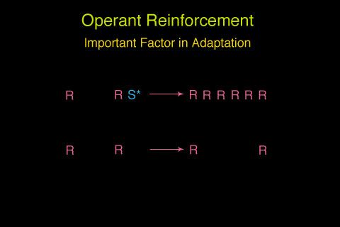 Slide 4
A critical factor in that adaptation is the occurrence of reinforcement.
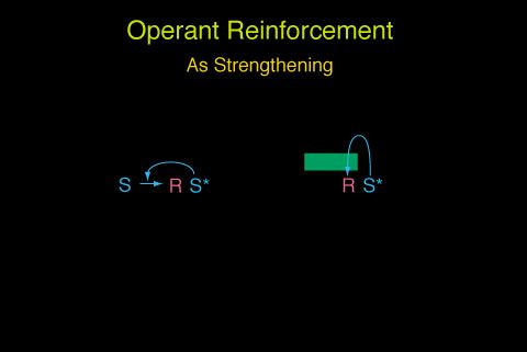 Slide 5
One way to conceptualize reinforcement is as something that strengthens a bond between a stimulus and a response or as something that strengthens a behavior in the presence of a stimulus.
 Slide 6
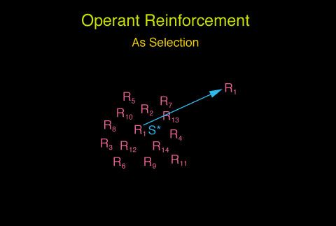
Alternatively, reinforcement can be seen as selecting one behavior out of many or as differentially strengthening one behavior rather than others.
 Slide 7
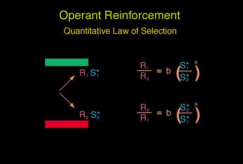
This general approach, that of seeing behavioral adaptation as one behavior coming to predominate over others can be formalized in a two alternative choice procedure. That is, how does one behavior come to predominate over another? This model of behavior has a quantitative specification of the probability of each behavior as a function of the available reinforcers.
 Slide 8
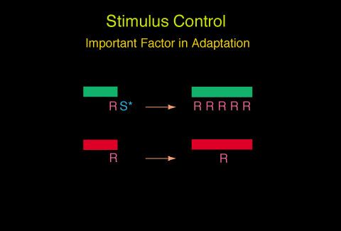
A second important fact in behavioral adaptation is stimulus control, that is, the stimulus in whose presence a behavior is reinforced comes to control that behavior on its future occurrences. Stimuli in whose presence behavior is not reinforced fail to control or suppress that behavior on their future occurrences.
 Slide 9
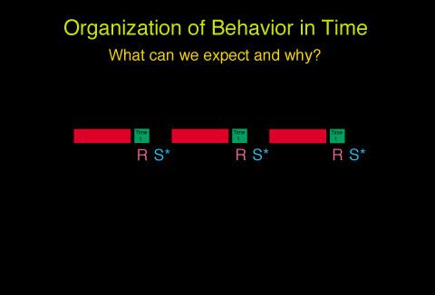
One example of stimulus control is temporal control. The temporal stimuli in effect at the moment of reinforcement would be expected to control responding. The temporal stimuli in effect when reinforcement does not occur would be expected to control nonresponding.
 Slide 10
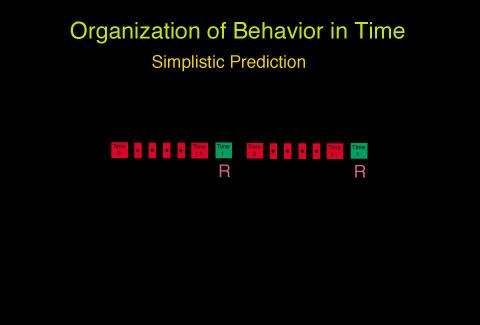
A simplistic prediction is, then, that a schedule with a temporal requirement such as one that reinforces the first peck following some fixed amount of time, should result in a single perfectly placed response.
 Slide 11
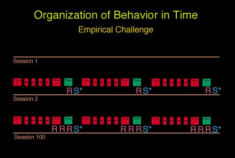
When empirically evaluated, this schedule does not produce the expected result. Rather, it controls responding across the entire latter portions of the interval rather than controlling only a single response.
 Slide 12
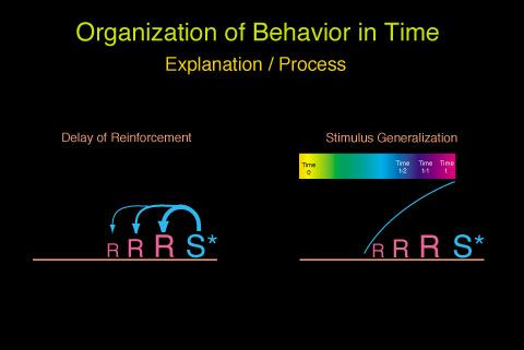
There are obvious candidates for why the simplistic prediction fails. Either reinforcement could strengthen more than just the last response, or the stimuli may be impossible to discriminate.
 Slide 13 (SLIDE WRONG)
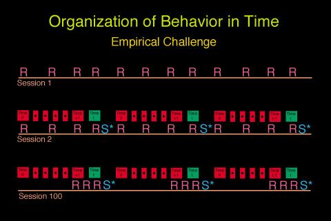
There is an empirical challenge to the indiscriminability hypothesis. If a short trial includes four stimuli, then responding occurs to only the last two stimuli. If the trial is lengthened by adding additional initial stimuli, then responding occurs to all four terminal stimuli. It is not plausible that those four stimuli become harder to distinguish as the result of a longer trial.
 Slide 14
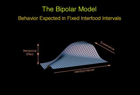
Palya has proposed a model based on the relative correlation with reinforcement of events in a repeating cycle. In a simple fixed interval, time in the interval is represented across the x axis, experience is represented back the z axis while vector, or strength of behavior is depicted on the y axis. (Note for purists: the axes had been rotated to maintain the dependent variable on the y axis.)
 Slide 15
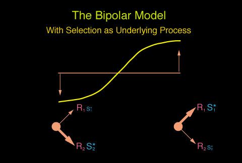
Palya has shown that strength and vector of the correlation between stimuli and food presentation control behaviors appropriate to that correlation. For example, stimuli correlated with the latter half of an interval are positively reinforcing while stimuli in the first half of an interval are negatively reinforcing. This bipolar view like Herrnstein, asserts that a fixed-interval schedule is, in effect, a concurrent schedule which systematically reverses its reinforcement ratio as the interval elapses.
 Slide 16
However, as Zeiler has aptly pointed out, any presumed process must be instantiated in an empirical procedure within at least 20 years of its articulation or it is nothing more than metaphysical speculation.
 Slide 17
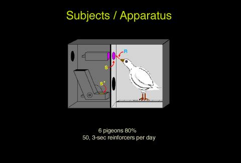
The present research used 6 pigeons at 80% ad lib and used 50, 3-sec food presentations (or that number just sufficient to maintain the birds at 80% body weight whichever was less).
 Slide 18
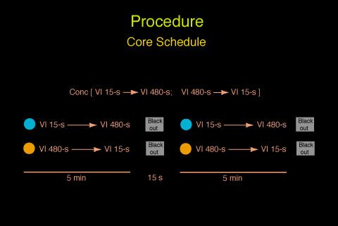
The basic schedule was a concurrent schedule in which the reinforcement ratio systematically varied from VI 15-sec / VI 480-sec to VI 480-sec / VI 15-sec over the course of a 5 minute trial. A 15-sec blackout intervened between trials.
 Slide 19
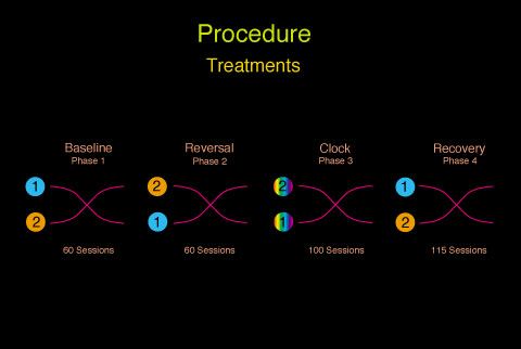
The four phases presented today are baseline, key reversal, added clock (which partitions the 10-min interval into ten distinct stimuli) and a recovery of baseline (i.e., JEAB Phases 1, 2, 3, 4, ----- Internal Phases 5, 6, 8, 13)
 Slide 20
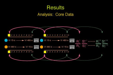
The basic analysis determines an average of the response and reinforcement ratios in each tenth of the trial. These are labeled synchronous averages in behavior dynamics because they are averages of bins synchronized with respect to some event; in this case, the beginning of the interval.
 Slide 21
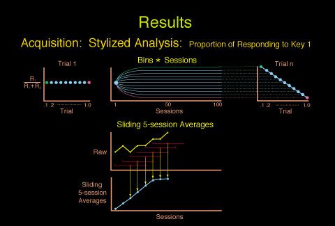
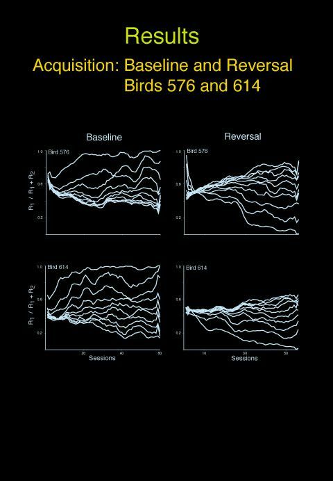
The "acquisition" measure indicates how responding in each tenth of the trial changes with increasing experience. The upper left frame shows equal response ratios in each tenth of the trial. The first tenth illustrated with a green dot, the last tenth illustrated with a red dot. The upper center frame shows an idealized acquisition where the successive tenths of the interval come to control from 100% to 0% responding on R1. The upper right frame shows the mean asymptotic behavior.
The bottom frame illustrates the sliding average procedure used. The raw data was smoothed with the same window typically used to index asymptotic behavior (i.e., 5 sessions). Session 3 on the lower smoothed figure is the average of sessions 1, 2, 3, 4, and 5. Session 4 is the average of 2, 3, 4, 5, 6, and so on. The first two and last two sessions do not have the same smoothing window. Session 1 on the lower plot includes only 1, 2, and 3. Session 2 includes only 1, 2, 3, and 4.
 Slide 22
This slide illustrates the original acquisition for two birds and the subsequent acquisition of a reversed baseline. (JEAB Phases 1, 2 / Internal Phases 5, 6)
 Slide 23
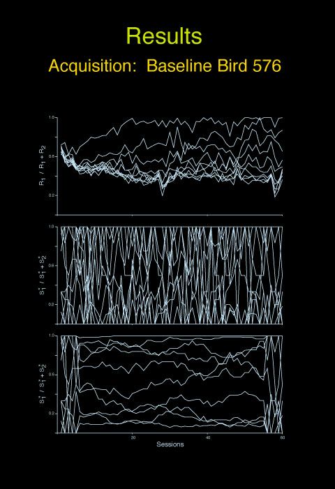
This slide illustrates the unsmoothed response functions (upper) and the unsmoothed (middle) and smoothed (lower) reinforcement functions. Note that the day-to-day reinforcement rates in each tenth of the trial are extremely variable. The 10-day smoothed averages more clearly differ. Clearly session averages of response rates were not as variable as session averages of reinforcement rates.
 Slide 24
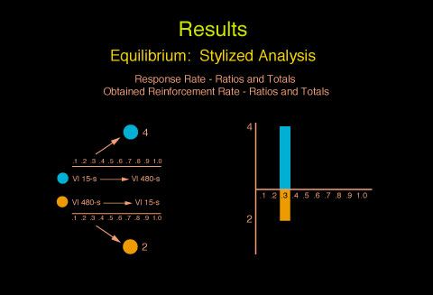
This figure shows how the asymptotic behavior was characterized. For example, the rates on each key in Bin 3 were plotted on a common axis with the rate to one key shown above the axis and the rate to the other key shown below the axis.
 Slide 25
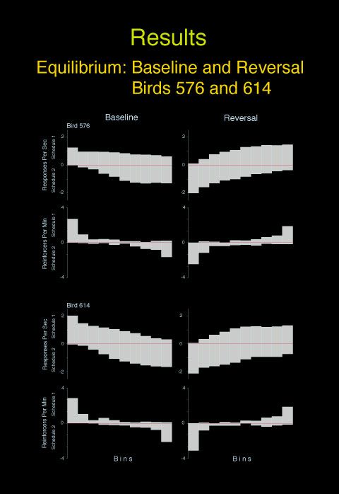
This figure shows the responding on each key for each bin and the reinforcement rates for each key for each bin. These data are for the baseline and subsequent reversal for Birds 576 and 614.
 Slide 26
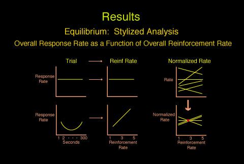
The overall reinforcement rate changed across the trial. It was lower in the middle of the interval. This figure illustrates how overall response rates were compared to overall reinforcement rates. For example, if the response rate were the same across the trial (upper left frame), then it would be flat as a function of changes in reinforcement rate (upper center) if the rate was U-shaped across the trial (lower left) then the response rate would increase as a function of reinforcement rate (lower center).
The right two panels show how the response rate changes as a function of reinforcement rate were normalized. The upper right frame shows the various functions for each of the six birds. These functions were normalized at the mean response rate at 2.5 reinforcers per minute for that group (lower right).
 Slide 27
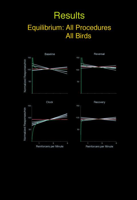
This slide shows the actual data from the six birds in each of the four phases. A flat function (red) is also included along with the best fit hyperbola (Green function). Note that two of the hyperbolas are negative and some birds have negative slopes (lower rates with higher reinforcement rates). Only the data in the clock provide evidence sympathetic with a hyperbolic relationship between overall reinforcement rate and overall response rate.
 Slide 28
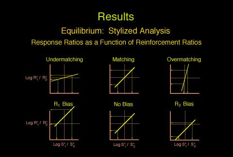
This stylized figure illustrates simple, clear ways to illustrate several relationships between response ratios and reinforcement ratios. The same response ratios as reinforcement ratios or matching is illustrated in the upper center. The upper left illustrates a split in behavior which is not as extreme, while the upper right illustrates a split in behavior which is more extreme than the reinforcement ratios. The bottom center frame illustrates no bias for either side, while the lower left and right frames illustrates a bias for R1 and R2, respectively.
 Slide 29
This slide illustrates the degree to which the allocation of responding in consecutive bins of the trial matched the allocations of reinforcers; across the whole trial (upper) across the first half(middle) and across the second half (bottom). Note that the second half of the trial did not control matching as well as the first half.
 Slide 30
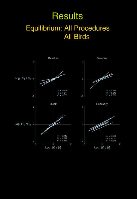
This slide illustrates the matching functions for all six birds for each of the four procedures. Note that the clock procedure resulted in superior matching.
 Slide 31
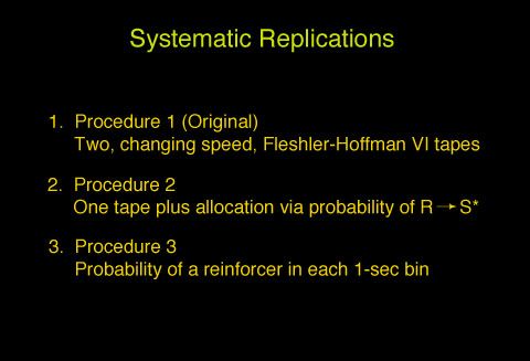
The general procedure of reciprocally interlocked dynamically changing concurrent schedules was replicated with two additional algorithms to insure that the obtained effect was not an artifact.
 Slide 32
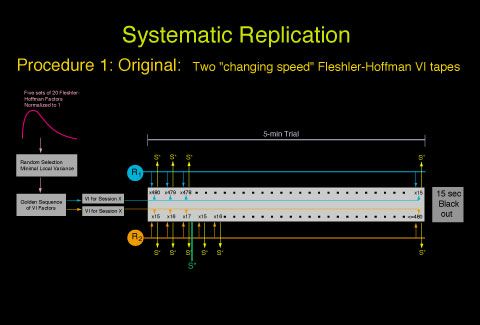
The original procedure, the one used in the prior four phases was implemented in the following way.
- Five sets of 20-element Fleshler-Hoffman factors normalized to one were generated.
- An algorithm which randomly selected the 100 factors without replacement was iteratively implemented until an ordering of the 100 factors was obtained which minimized the sample-to-sample variance when the sample contained 12 elements. This arrangement of the 100 factors was labeled the "golden VI tape."
- An independent random starting point was selected for each of the two concurrent schedules for each session. Factors were subsequently drawn from the golden tape in sequential order.
- A VI 480-sec schedule, for example, was implemented by multiplying the VI factor by 480 which over repeated factors produced a VI 480-sec schedule. The other schedules were implemented by multiplying the VI factors by the term which resulted in the desired schedule.
- The parameter value for each schedule continuously changed across the 5-min trial, so that the first key ended with a VI 15-s schedule and the other key ended with a VI 480-s schedule. These schedules were programmed by determining if the IRI at the instant a peck occurred exceeded the required IRI for that side at that instant. If the appropriate schedule at that instant was a VI 60-s, for example, then the IRI factor from the golden tape which was in effect was multiplied by 60. If the time since the last reinforcer exceeded the required IRI, a reinforcer occurred; if not, then no consequence followed that peck. The VI schedule parameter (i.e., a value between 15 and 480) was determined at the temporal position of the end of the current IRI on the improving schedule and at the beginning of the IRI on the worsening schedule.
JEAB Phases 1, 2, 3, 4 Internal Phases 5 through 13
 Slide 33
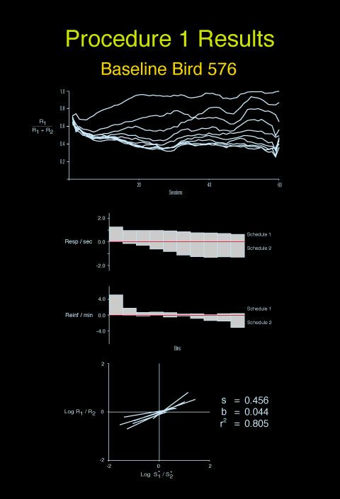
This figure illustrates the acquisition (upper), the response and reinforcement rates for each key in each bin (center), and the matching functions (lower) under this procedure for Bird 576.
 Slide 34
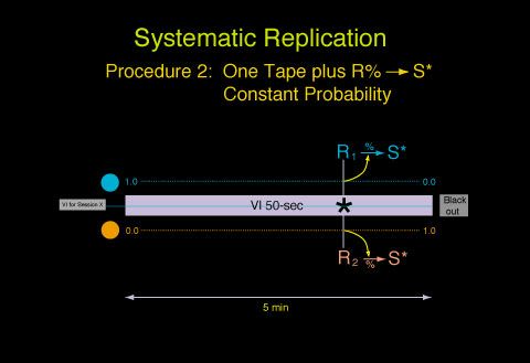
This is a diagram of the procedure used in the first replication. In this case, values were drawn in order, from the golden VI factors following a randomly selected starting point and multiplied by the term that would produce a VI 50-sec. When reinforcement "set up", it was assigned to the left or right key in a reciprocally interlocked changing schedule such that at the beginning of the trial, the probabilities were 1, and 0, and at the end of the trial the probabilities were 0 and 1.
JEAB Phase 5 Internal Phases 14, 15, 16
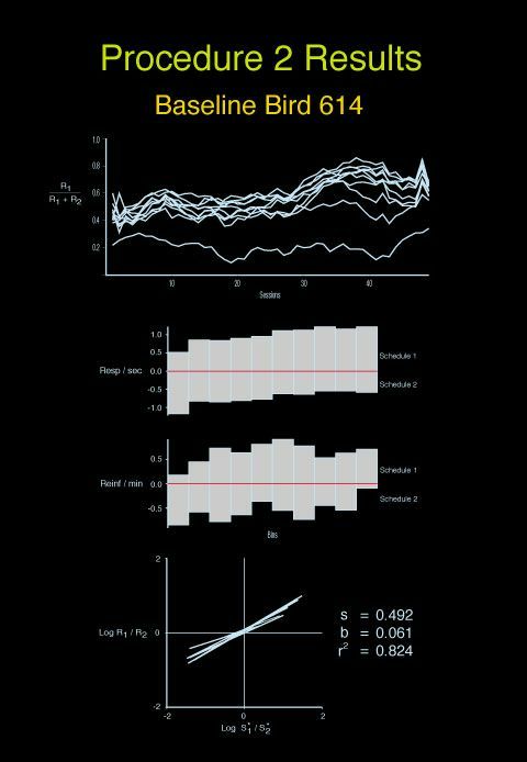 Slide 35
This figure depicts the acquisition (upper), the response and reinforcement rates (middle), and the matching functions (lower) for Bird 614 under this procedure. (It was an accident that different birds had been used in Slide 33 and Slide 35)
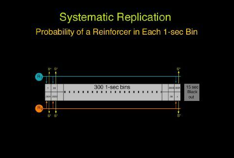 Slide 36
The third replication partitioned the 5-min trial into 300, 1-sec bins and probabilistically reinforced each response on each key on a reciprocally interlocked changing schedule. Additional data on a similar procedure, which is not included in the paper or in this web appendix is available from Bob Allan at Lafayette College.
JEAB Phases 6 and 7 Internal Phases 17 and 18
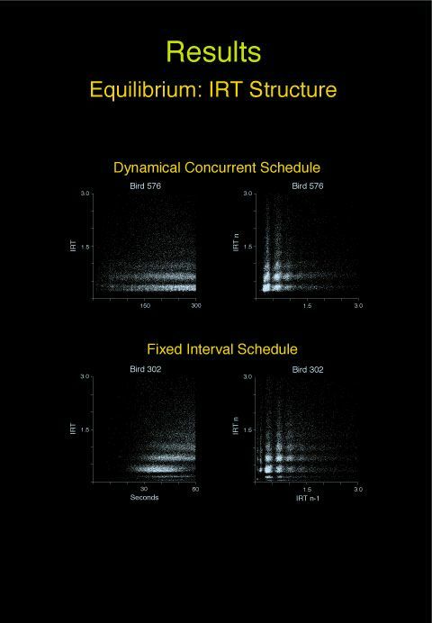 Slide 37
This is a dot plot of the IRTs as a function of time in the interval and as a function of IRT n-1. The figure compares a bird under a traditional fixed interval schedule and under the dynamically changing reciprocally interlocked concurrent schedule.
Out-takes / Extras
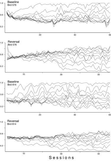 Figure 100
Unsmoothed acquisition and reversal. Phases 5 and 6 for Birds 576 and 614. See JEAB Figure 2 and Web Slide Set Figures 21 and 22 for related information and explanation.
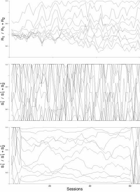 Figure 101
Unsmoothed response rates and unsmoothed and smoothed reinforcement rates, Phase 5, Bird 614. See JEAB Figure 2 and Web Slide Set Figures 21 and 23. Note ten session smoothing was used on reinforcement rates. That results in an apparent change in the variability of the ten functions at the left and right edge of the figure.
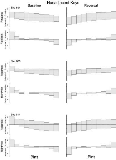 Figure 102
Equilibrium response rates for nonadjacent keys Phases 5 and 6. See Slide Set 24 and 25 and JEAB Figure 4
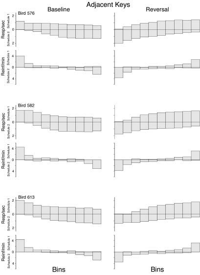 Figure 103
Equilibrium response rates for adjacent keys Phases 5 and 6. See JEAB Figure 1 and Web Slide Set Figures 24 and 25 and JEAB Figure 4.
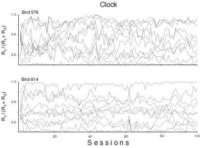 Figure 104
Rate in each bin as a function of session number in clock phase. See Slides 21, 22, 23 and JEAB Figures 2, 6, 7.
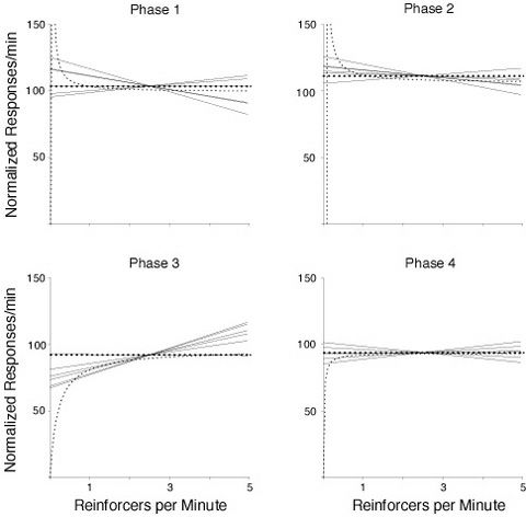 Figure 105
Rate as a function of reinforcer rate and the best fit hyperbola. See Slides 26 and 27.
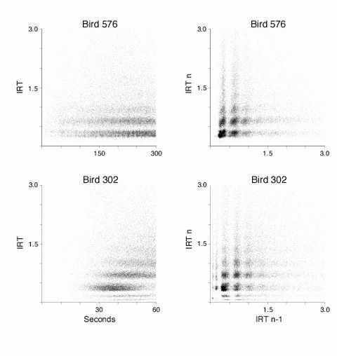 Figure 106
Obtained IRT structure and that of a bird under a typical schedule. See Slide 37 and JEAB Figure 10.
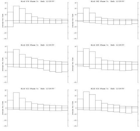 Figure 107 Dwell Phase 5
(JEAB 1)
Figure 107 Dwell Phase 5
(JEAB 1)
Dwell. The mean of all runs (peck stream uninterrupted by peck to other key) that intersected a bin are depicted for each bin for each key.
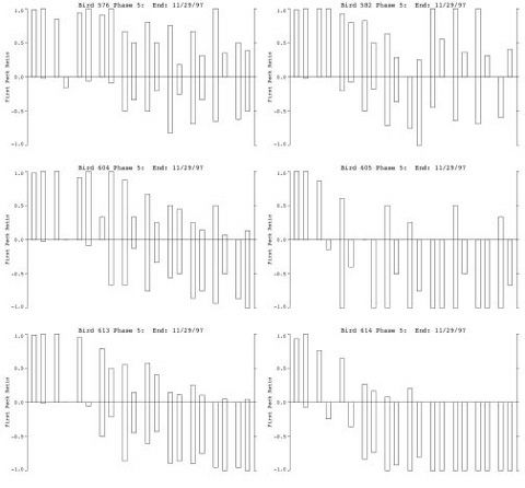 Figure 108 First peck Phase 5
(JEAB 1)
Figure 108 First peck Phase 5
(JEAB 1)
First Peck. Four bars are presented for each bin. The two bars above the x axis for a bin depict data for Schedule 1 (the first peck following a reinforcer was on key 1). The two bars below the x axis depict data for Schedule 2 (the first peck following a reinforcer was on Key 2). The first bar in each pair depicts first pecks that were on the same side as the reinforcer. The second bar in each pair depicts first pecks that were on the side opposite to that of the reinforced key peck. Note that proportions are provided on the y axis.
When considering the four bars for each bin, for example, the upper left, depicts the percentage of first pecks which were on Key 1 following a Key 1 reinforcer. The upper right depicts the percentage of first pecks which were on Key 1 following a Key 2 reinforcer. The height of the bars indicate the proportion of total first pecks in that category. The upper left and lower right (and lower left and upper right) bars of each group necessarily sum to 1.
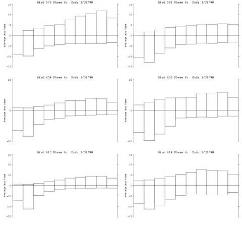 Figure 109 Dwell Phase 6.
(JEAB 2)
Figure 109 Dwell Phase 6.
(JEAB 2)
The mean of all runs (peck stream uninterrupted by peck to other key) that intersected a bin are depicted for each bin for each key.
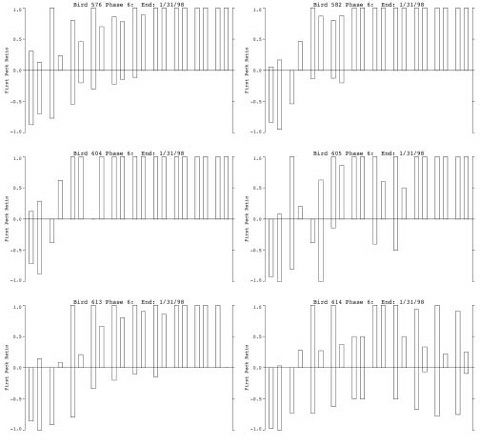 Figure 110 First Phase 6.
(JEAB 2)
Figure 110 First Phase 6.
(JEAB 2)
Four bars are presented for each bin. The two bars above the x axis depict data for Schedule 1 (the first peck following a reinforcer was on key 1). The two bars below the x axis depict data for Schedule 2 (the first peck following a reinforcer was on Key 2). The first bar in each pair depicts first pecks that were on the same side as the reinforcer. The second bar in each pair depicts first pecks that were on the side opposite to that of the reinforced key peck.
For example, the upper left, depicts the percentage of first pecks which were on Key 1 following a Key 1 reinforcer. The upper right depicts the percentage of first pecks which were on Key 1 following a Key 2 reinforcer. The height of the bars indicate the proportion of total first pecks in that category. The upper left and lower right (and lower left and upper right) bars of each group necessarily sum to 1.
 Figure 111 Dwell Phase 8. (JEAB 3)
The mean of all runs (peck stream uninterrupted by peck to other key) that intersected a bin are depicted for each bin for each key.
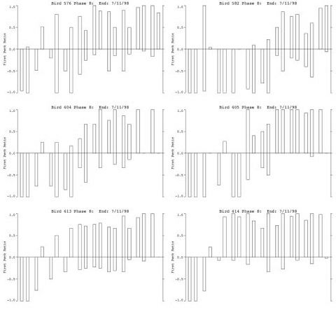 Figure 112 First Phase 8.
(JEAB 3)
Figure 112 First Phase 8.
(JEAB 3)
Four bars are presented for each bin. The two bars above the x axis depict data for Schedule 1 (the first peck following a reinforcer was on key 1). The two bars below the x axis depict data for Schedule 2 (the first peck following a reinforcer was on Key 2). The first bar in each pair depicts first pecks that were on the same side as the reinforcer. The second bar in each pair depicts first pecks that were on the side opposite to that of the reinforced key peck.
For example, the upper left, depicts the percentage of first pecks which were on Key 1 following a Key 1 reinforcer. The upper right depicts the percentage of first pecks which were on Key 1 following a Key 2 reinforcer. The height of the bars indicate the proportion of total first pecks in that category. The upper left and lower right (and lower left and upper right) bars of each group necessarily sum to 1.
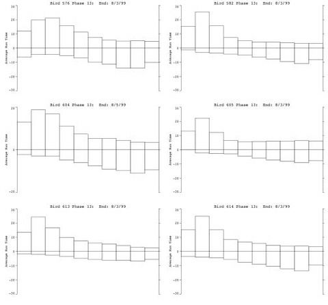 Figure 113 Dwell Phase 13.
(JEAB 4)
Figure 113 Dwell Phase 13.
(JEAB 4)
The mean of all runs (peck stream uninterrupted by peck to other key) that intersected a bin are depicted for each bin for each key.
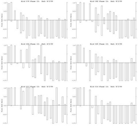 Figure 113 First Phase 13.
(JEAB 4)
Figure 113 First Phase 13.
(JEAB 4)
Four bars are presented for each bin. The two bars above the x axis depict data for Schedule 1 (the first peck following a reinforcer was on key 1). The two bars below the x axis depict data for Schedule 2 (the first peck following a reinforcer was on Key 2). The first bar in each pair depicts first pecks that were on the same side as the reinforcer. The second bar in each pair depicts first pecks that were on the side opposite to that of the reinforced key peck.
For example, the upper left, depicts the percentage of first pecks which were on Key 1 following a Key 1 reinforcer. The upper right depicts the percentage of first pecks which were on Key 1 following a Key 2 reinforcer. The height of the bars indicate the proportion of total first pecks in that category. The upper left and lower right (and lower left and upper right) bars of each group necessarily sum to 1.
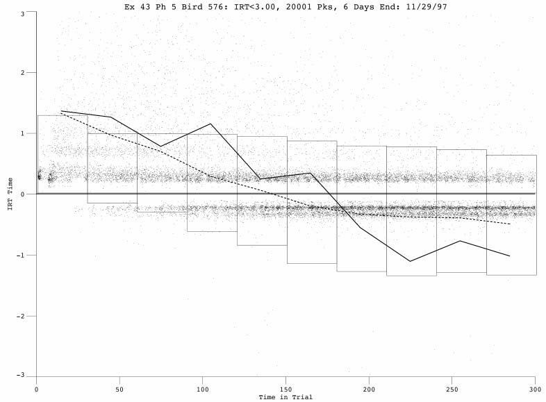
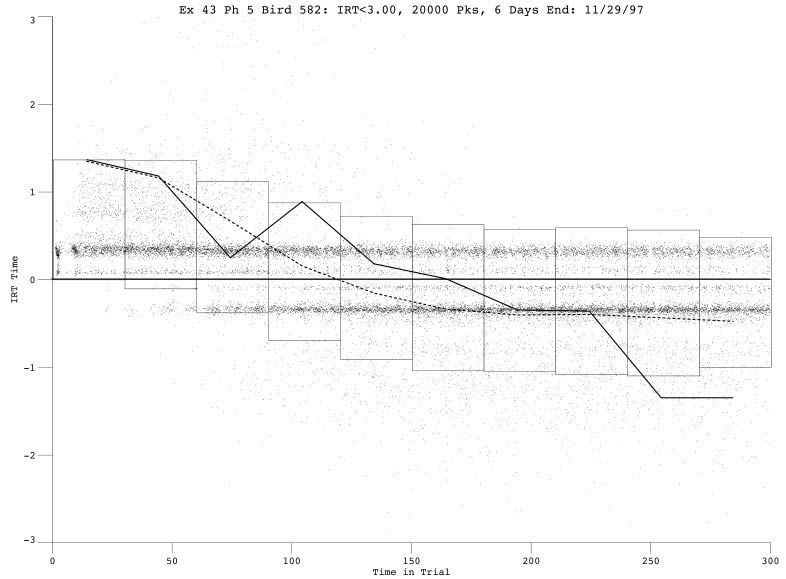
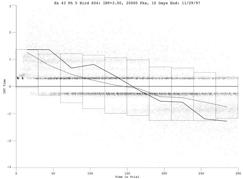
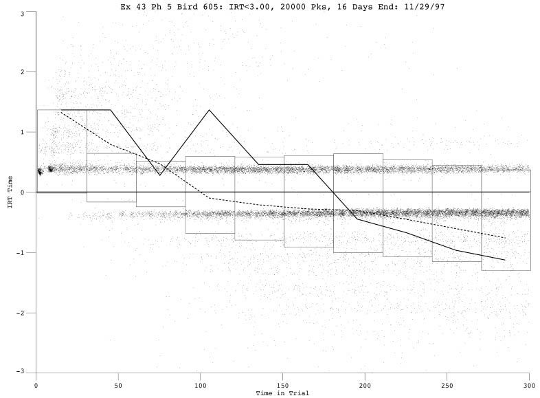
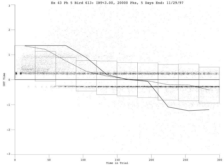
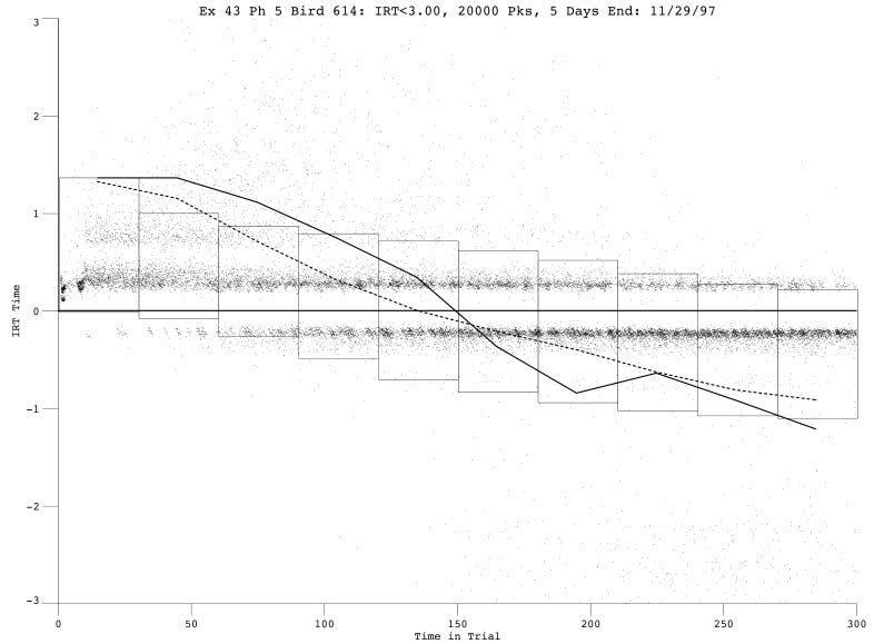
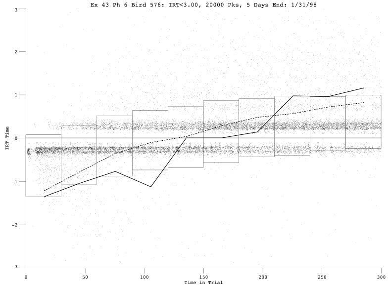
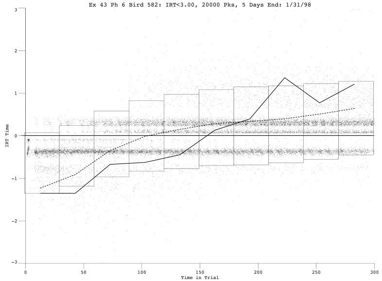
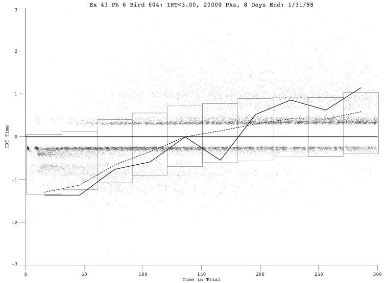
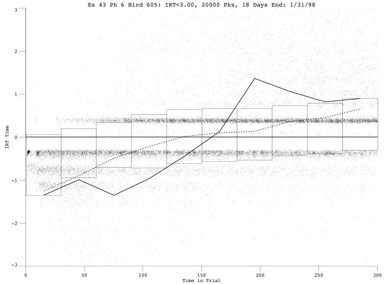
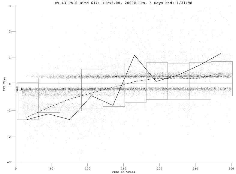
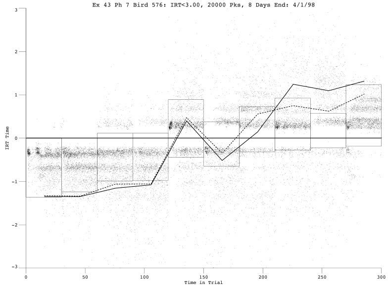
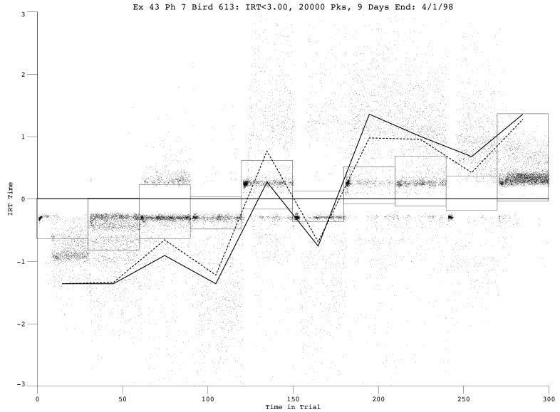
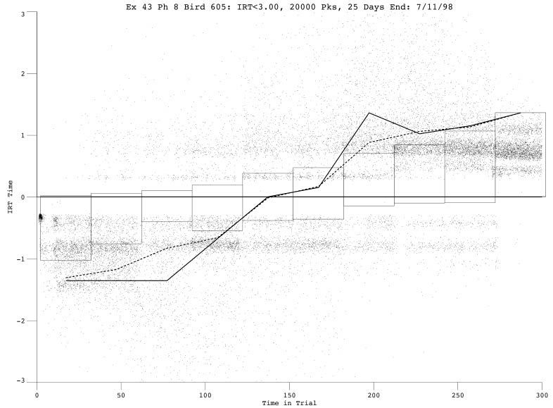
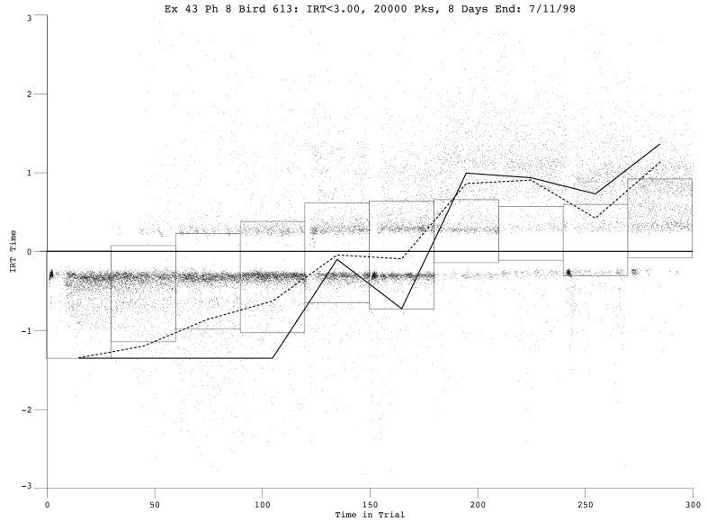
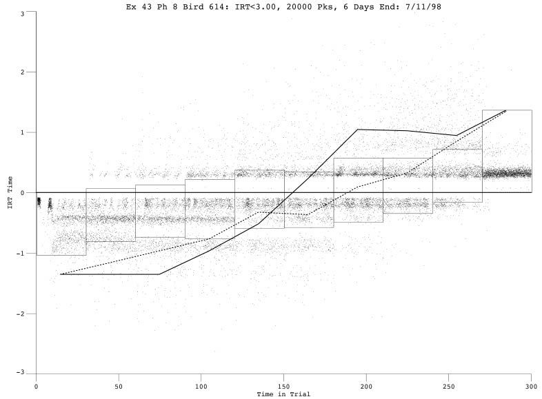
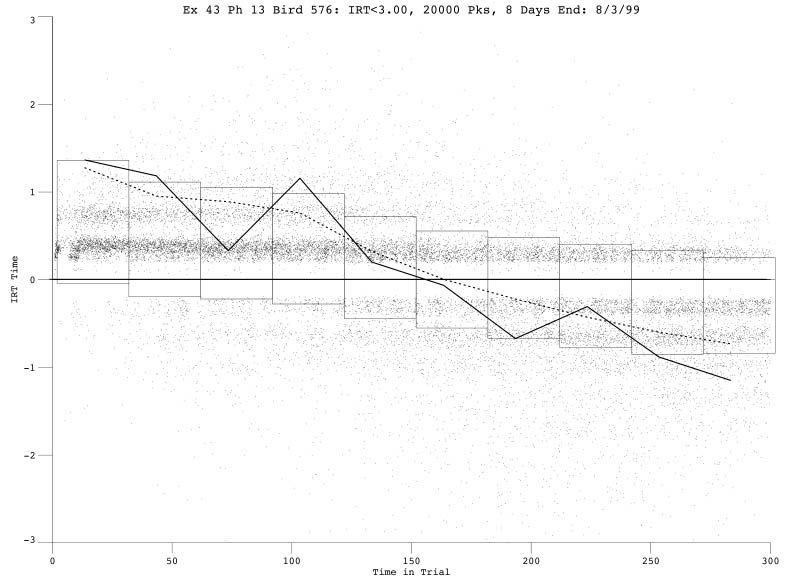
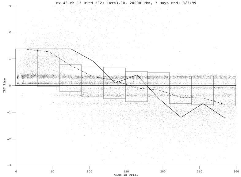
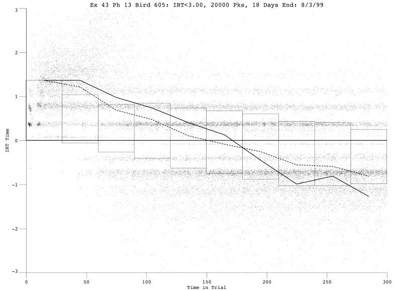
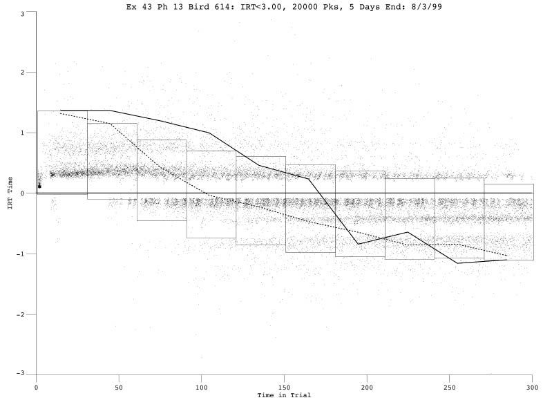
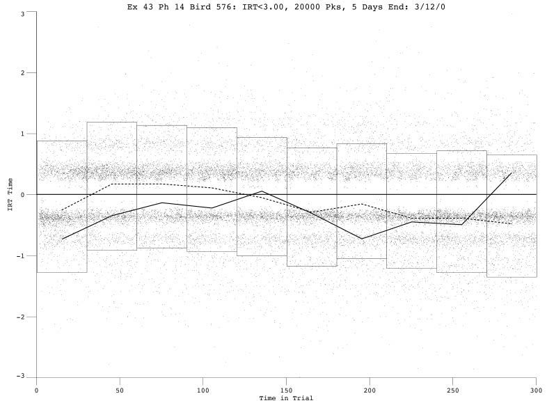
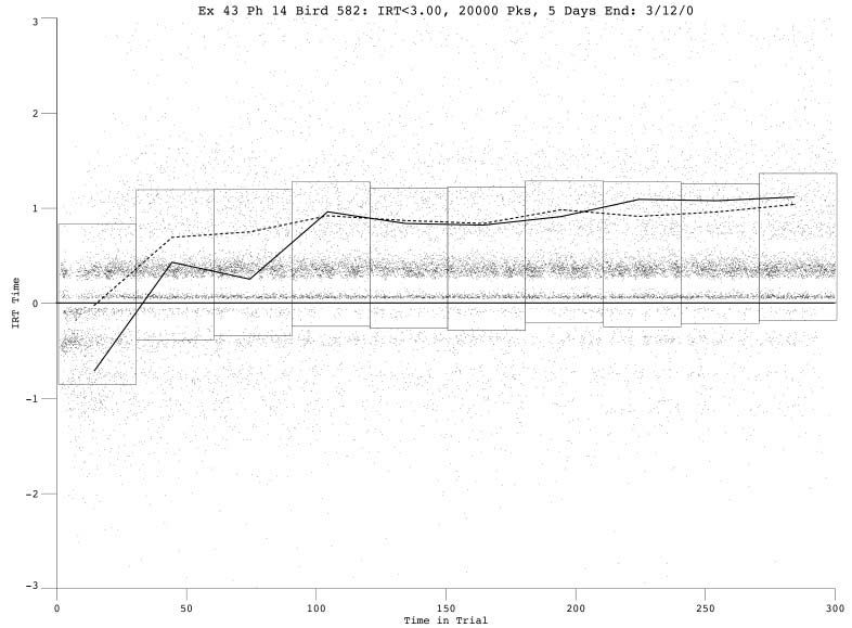
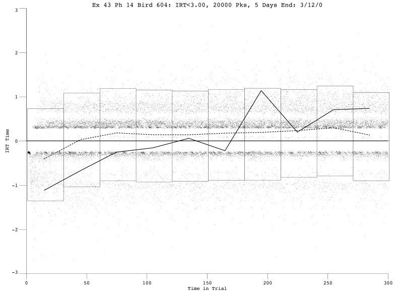
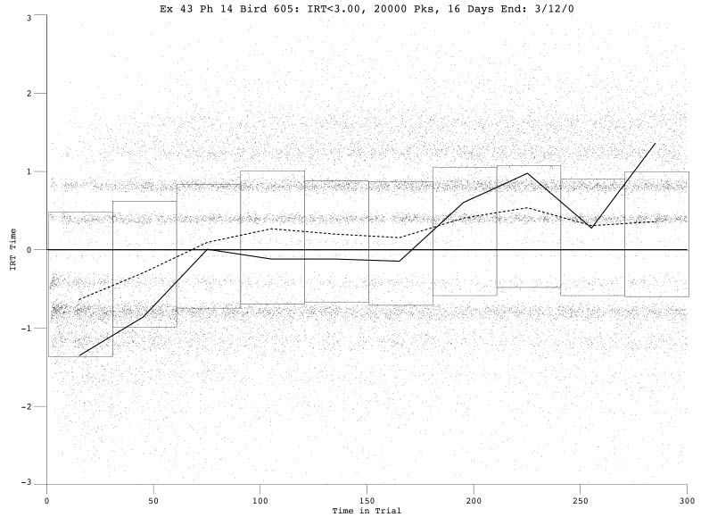
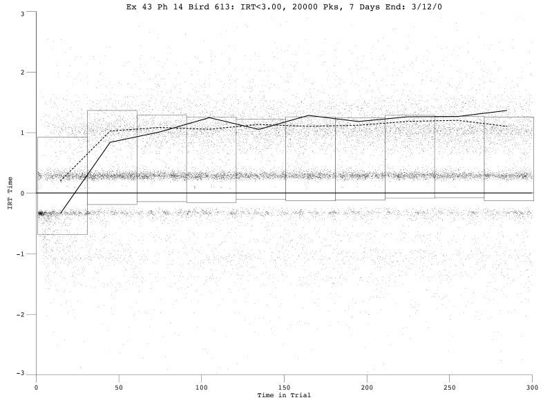
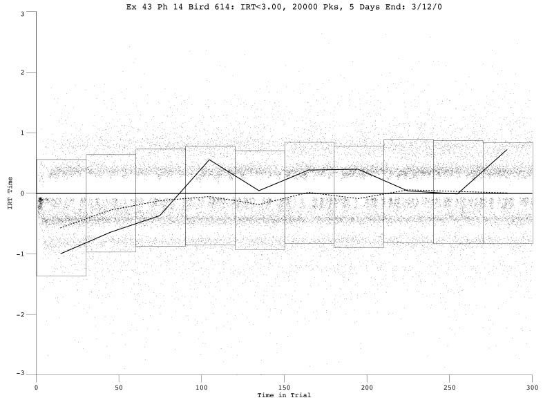
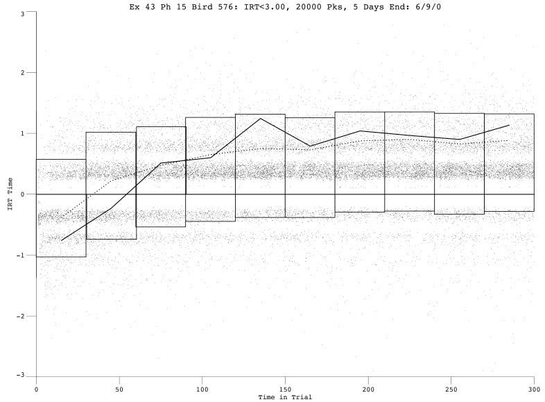
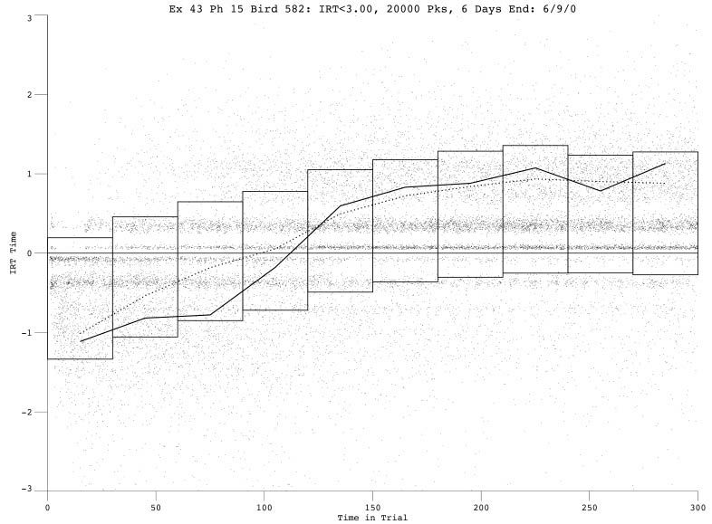
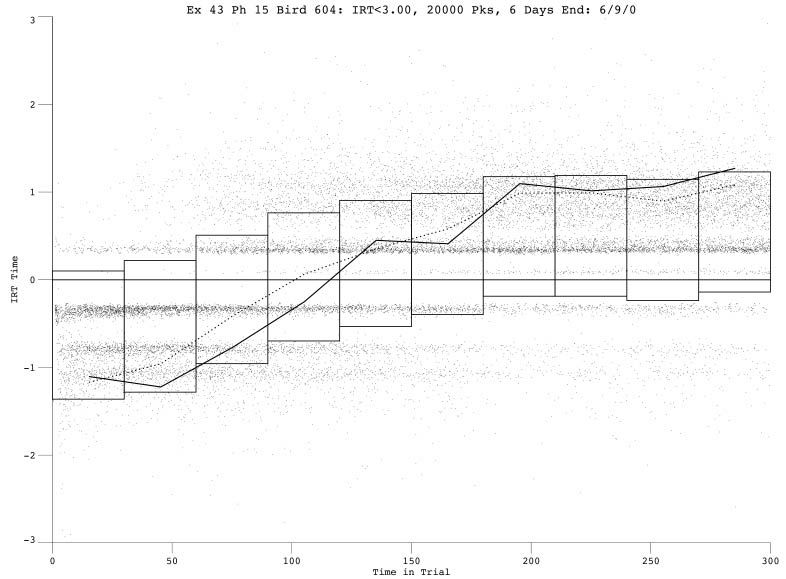
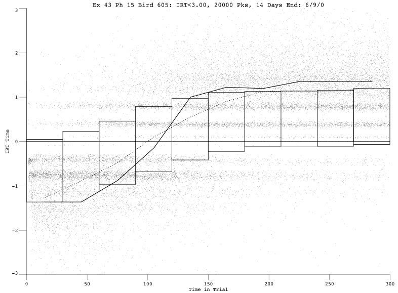
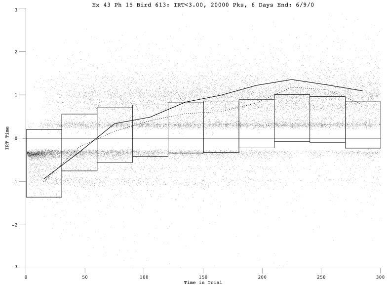
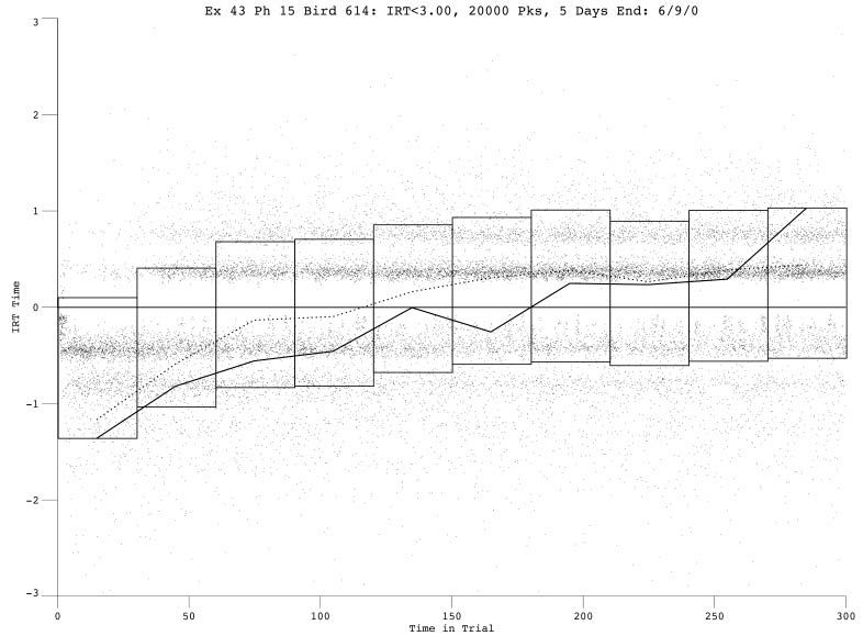
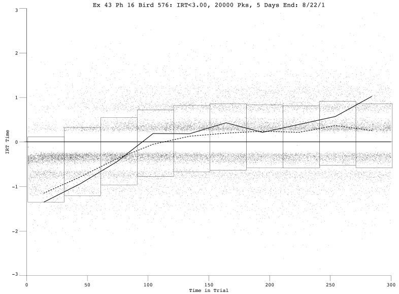
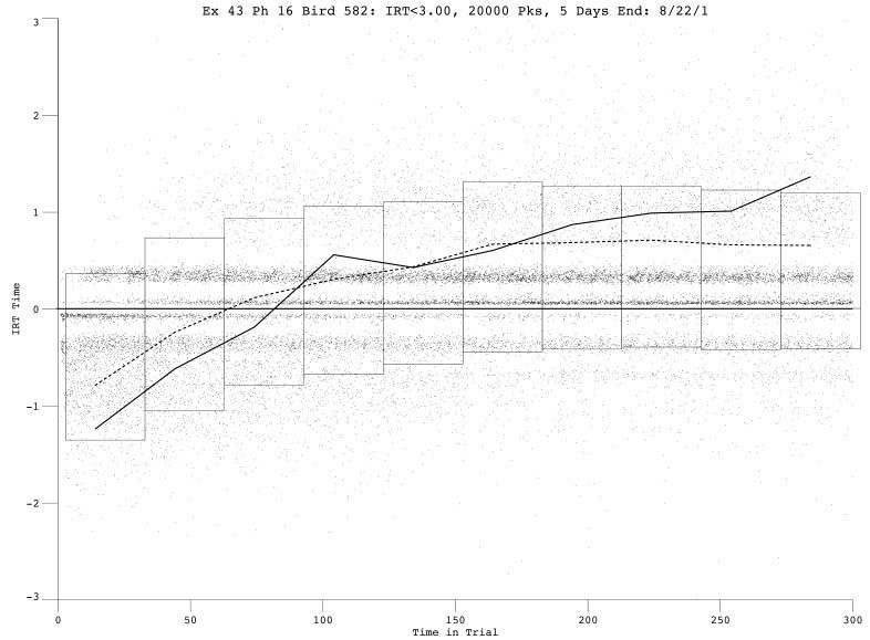
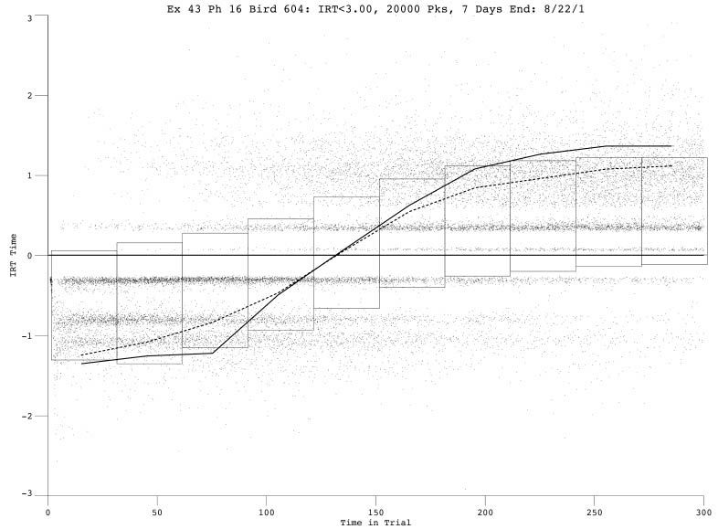
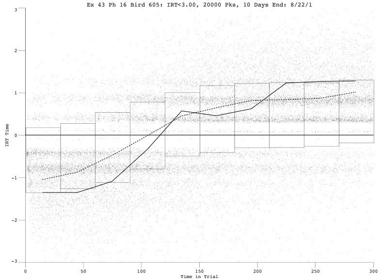
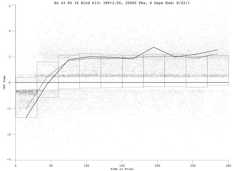
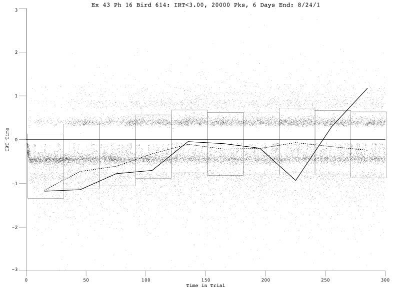
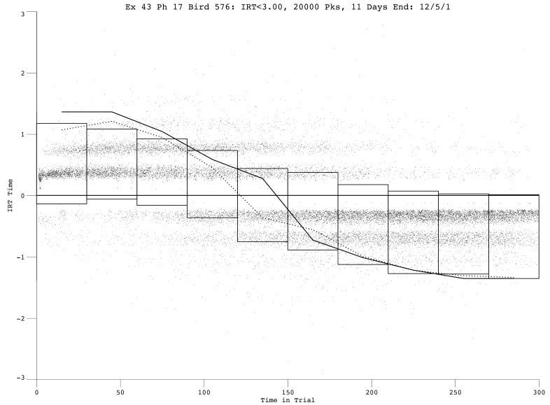
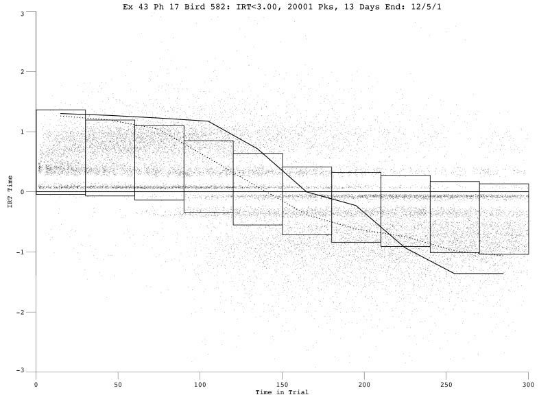
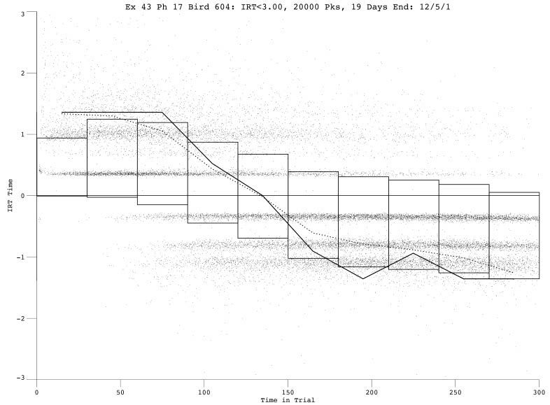
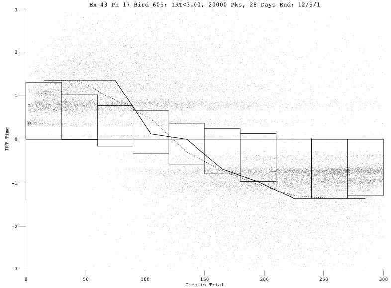
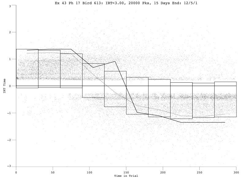
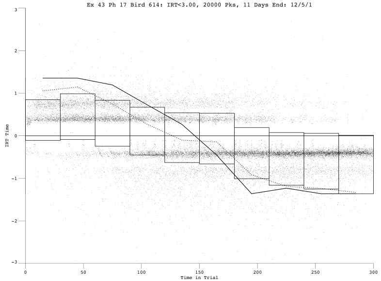
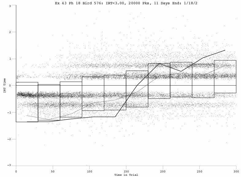
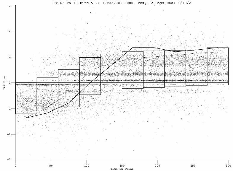
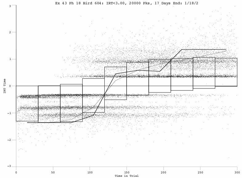
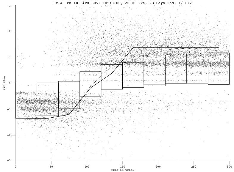
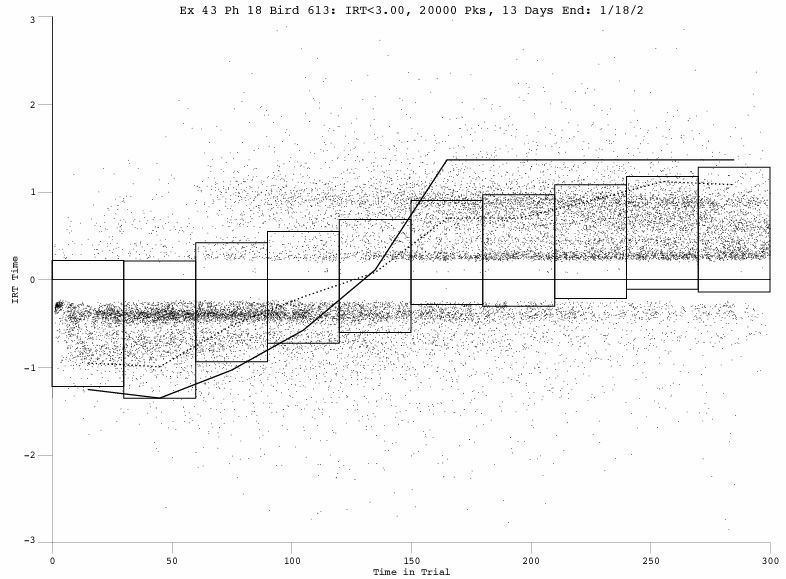
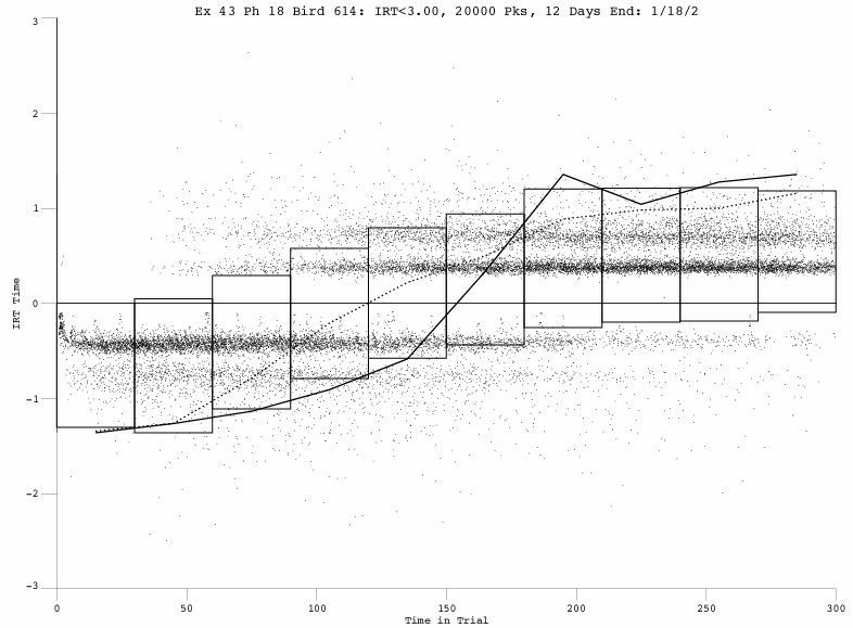
The following table provides figures for each bird and for each phase. We will add the missing phases as soon as we get time. They provide the following information.
The Dots: The IRT structure across the trial for each key (above and below the x axis).
See JEAB Figure 5 and Palya 1992 Figure 6
The Histograms: The equilibrium response rates in each bin for each key (above and below the x axis)
See JEAB Figure 6 and Web Slides 24 and 25
The Dotted Line: The response ratio R1 / (R1+R2) for each bin across the trial. See Web Slides 20 and 21 (but in this case, it is only the frame in the upper right)
The Solid Line: The reinforcement ratio S*1 / (S*1 +S*2) for each bin across the trial. See Web Slides 20 and 21 (but in this case, it is only the frame in the upper right, but with bin-by-bin reinforcement rate rather than response rate)
| Phase | Birds | ||||||
| 576 | 582 | 604 | 605 | 613 | 614 | ||
| 5 | (JEAB 1) | ||||||
| JPEG | JPEG | JPEG | JPEG | JPEG | JPEG | ||
| 6 | (JEAB 2) | ||||||
| JPEG | JPEG | JPEG | JPEG | JPEG | JPEG | ||
| 7 | |||||||
| JPEG | JPEG | JPEG | JPEG | JPEG | JPEG | ||
| 8 | (JEAB 3) | ||||||
| JPEG | JPEG | JPEG | JPEG | JPEG | JPEG | ||
| 9 | PDF Missing | PDF Missing | PDF Missing | PDF Missing | PDF Missing | PDF Missing | |
| JPEG | JPEG | JPEG | JPEG | JPEG | JPEG | ||
| 10 | PDF Missing | PDF Missing | PDF Missing | PDF Missing | PDF Missing | PDF Missing | |
| JPEG | JPEG | JPEG | JPEG | JPEG | JPEG | ||
| 11 | PDF Missing | PDF Missing | PDF Missing | PDF Missing | PDF Missing | PDF Missing | |
| JPEG | JPEG | JPEG | JPEG | JPEG | JPEG | ||
| 12 | PDF Missing | PDF Missing | PDF Missing | PDF Missing | PDF Missing | PDF Missing | |
| JPEG | JPEG | JPEG | JPEG | JPEG | JPEG | ||
| 13 | (JEAB 4) | ||||||
| JPEG | JPEG | JPEG | JPEG | JPEG | JPEG | ||
| 14 | (JEAB 5) | ||||||
| JPEG | JPEG | JPEG | JPEG | JPEG | JPEG | ||
| 15 | (JEAB 5) | ||||||
| JPEG | JPEG | JPEG | JPEG | JPEG | JPEG | ||
| 16 | |||||||
| JPEG | JPEG | JPEG | JPEG | JPEG | JPEG | ||
| 17 | (JEAB 6) | ||||||
| JPEG | JPEG | JPEG | JPEG | JPEG | JPEG | ||
| 18 | (JEAB 7) | ||||||
| JPEG | JPEG | JPEG | JPEG | JPEG | JPEG | ||
Some Day If There Is Interest
The following figures are the "dailies." They present the response rate in each tenth of the trial for each consecutive day. They depict acquisition and day-to-day stability. Our standard lab protocol uses that type of presentation to evaluate stability for phase change decisions. We will put them up when we get time, if there is interest.
See JEAB Figure 2 and Web Slides Figures 20, 21, 22 and 23.
| Phase | Birds | |||||
| 576 | 582 | 604 | 605 | 613 | 614 | |
| 5 | ||||||
| JPEG | JPEG | JPEG | JPEG | JPEG | JPEG | |
| 6 | ||||||
| JPEG | JPEG | JPEG | JPEG | JPEG | JPEG | |
| 7 | ||||||
| JPEG | JPEG | JPEG | JPEG | JPEG | JPEG | |
| 8 | ||||||
| JPEG | JPEG | JPEG | JPEG | JPEG | JPEG | |
| 9 | ||||||
| JPEG | JPEG | JPEG | JPEG | JPEG | JPEG | |
| 10 | ||||||
| JPEG | JPEG | JPEG | JPEG | JPEG | JPEG | |
| 11 | ||||||
| JPEG | JPEG | JPEG | JPEG | JPEG | JPEG | |
| 12 | ||||||
| JPEG | JPEG | JPEG | JPEG | JPEG | JPEG | |
| 13 | ||||||
| JPEG | JPEG | JPEG | JPEG | JPEG | JPEG | |
| 14 | ||||||
| JPEG | JPEG | JPEG | JPEG | JPEG | JPEG | |
| 15 | ||||||
| JPEG | JPEG | JPEG | JPEG | JPEG | JPEG | |
| 16 | ||||||
| JPEG | JPEG | JPEG | JPEG | JPEG | JPEG | |
| 17 | ||||||
| JPEG | JPEG | JPEG | JPEG | JPEG | JPEG | |
| 18 | ||||||
| JPEG | JPEG | JPEG | JPEG | JPEG | JPEG | |
 Back to SEBAC Welcome Page
Last Reviewed : November 16, 2002