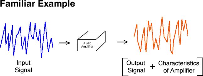
Most people are familiar with the characterization of the output of an audio amplifier (e.g., sound from a speaker) as the input signal (e.g., a microphone) plus amplification and distortion.
Basic Idea
Most people are familiar with the characterization of the output of
an audio amplifier (e.g., sound from a speaker) as the input signal (e.g.,
a microphone) plus amplification and distortion.

The productive use of that concept (i.e., that behavior is the input plus the characteristics of the organism) is mathematically complex. The complexity can be dramatically simplified by carrying out the numerical operations necessary to predict behavior in a different domain. Most people are familiar with a similar domain conversion to simplify a problem.
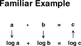
The multiplication of two numbers can be simplified to the addition
of the logs of those two numbers. The result (in the example "log
C") is simply converted back to the original domain by taking the antilog.
This is the principle underlying "slide rulers" which were used by engineers
before hand-held calculators.
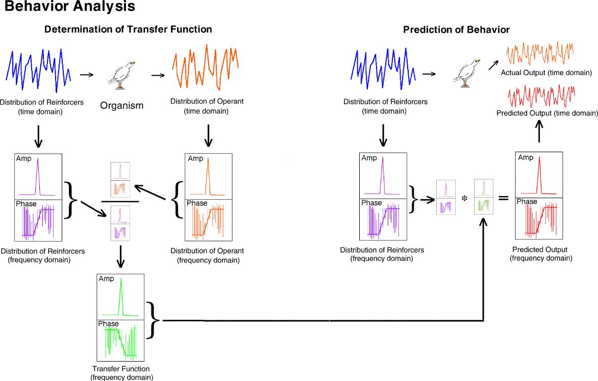
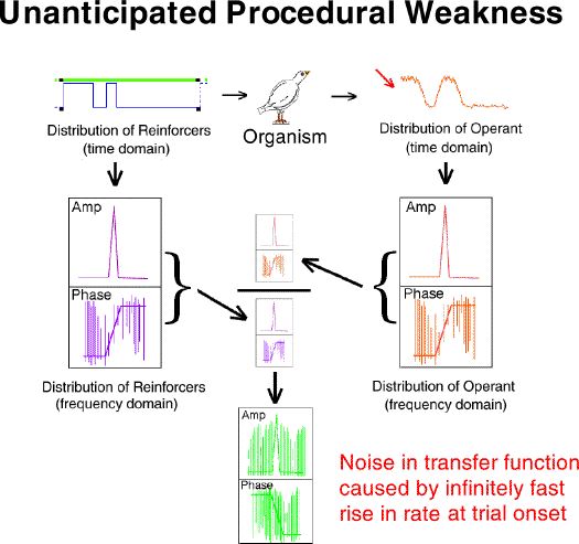
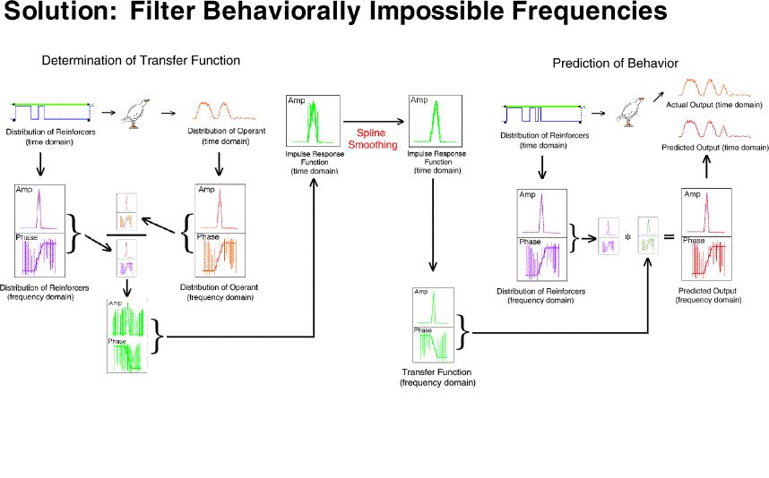
The steps are as follows. [left side] (blue upper left) the distribution
of reinforcers provided to the organism (e.g., a 20-element Fleshler-Hoffman
series with a mean of 60 seconds) is translated into the frequency domain
(purple middle left). Note that the conversion produces a set of
values for both amplitude at each frequency and phase. The output
behavior of the organism which occurs as the result of that VI schedule
input (orange upper right) is translated into the frequency domain (amber
middle right).
The frequency domain output (amber middle right) is divided by
the frequency domain input (purple middle right). The result is the
frequency domain transfer function (green bottom center).
Subsequently, [right side] any input (blue upper left) can be
converted to the frequency domain (purple middle) multiplied by the previously
obtained transfer function. This results in a predicted output in
the frequency domain (red middle right). This prediction can then be converted
to the time domain (red upper right) and compared to the actual behavior
(orange upper right).
We have already exposed birds to the necessary procedures, worked out the various procedural and numerical methods; and compared the obtained predictions to those obtained with actual organisms under novel test conditions.
The following panel presents a review of the rationale for the procedure, the actual experimental procedure, and the obtained results.

The first task of obtaining a useful transfer function for an audio
amplifier or an organism is to expose the system to all possible frequencies.
In that way, a prediction can be made for the subsequent exposure to any
possible combination of any possible input frequencies. Obviously
a brute force presentation of each frequency would be very time consuming.
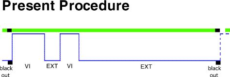
The trick is to take advantage of the fact that a simple square wave or
a "step function" actually contains all possible frequencies (proven by
Fourier�s theorem). So if an organism is exposed to a VI 20" schedule
for 200 seconds followed by extinction for 800 seconds, for example, then
that is the same as presenting to that organism a whole series of different
input frequencies individually. This is in fact precisely what we
did.
The procedure is illustrated in the middle of the figure.
It was shown that reasonable, zero-free parameter predictions could
be made based on the use of a transfer function obtained with this procedure.
It is important to reiterate that no scaling adjustments are used with
this method. It is truly a zero free parameter prediction.
While it was shown that the conceptual machinery would work, the predictions
were not perfect. Our current research in this area is intended to
further reduce the error of prediction caused by noise by developing better
experimental procedures and better analytical and numerical methods.
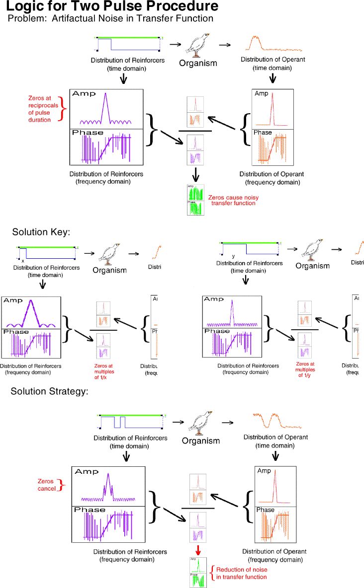
The top portion of this frame illustrates a major source of artifactual
noise in the determination of a transfer function with a step transition.
Division at each of the multiples of the reciprocals of the input step
transition pulse duration is impossible because they are zero. The
loss of data at these points results in a noisy transfer function.
There is a solution to this problem. It is illustrated in the
"solution key" section of the figure. If the zeros occur at reciprocals
of the pulse duration, then different pulse durations have zeros at different
points. Exposing an organism to a two-pulse procedure would result
in the cancellation of the zeros in the frequency domain version of the
input because valid data is provided by one pulse duration or the other
at every point across the spectrum. This is precisely what we did.
Present Research Prediction of Behavior
One of the great benefits of this analytical approach to behavior analysis is that it gives us a way to understand one of the most fundamental questions in the analysis of behavior. A familiar example of this issue is given by bandpass filters.
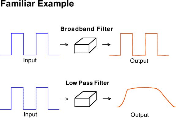
A broad-band filter passes all the details (both sharp edges and slow
trends) of the input signal. An audio amplifier is better if it passes
all of these details. A low pass filter on the other hand, would
blur all the fine details and give only the broad averages. A very
inexpensive or low fidelity amplifier is said to have a poor "frequency
response" because of its poor band pass characteristics.
This difference can be more usefully seen as the filter characteristics of the organism (e.g., broad-band versus low-pass). The importance of this relabeling is that it connects us to an enormous body of conceptual and analytical tools used to great benefit by "older" sciences.
The great power of a transfer function analysis is that it will predict
a zero free parameter output for any possible input. It will specify
the precise filter characteristics for particular organisms in particular
situations given even complex input signals.
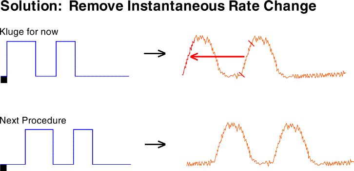
As a kluge for one bird (because there was no time to collect data
for a new transfer function and include it in the scheduled poster session)
we simply copied the gradual rate increase from the second slope to the
first slope. This eliminated that source of noise.
Our current solution is to use a procedure which does not result in
an instantaneous, large magnitude rate change. The first VI pulse
is offset from the trial start so that behavior will not instantaneously
change to a high rate.
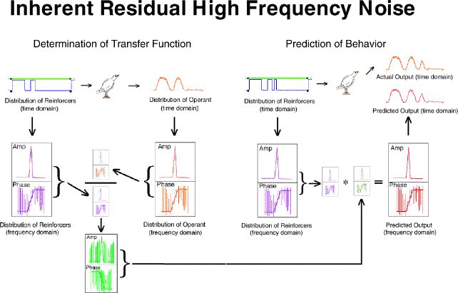
As a second noise reduction technique we converted the transfer function
(frequency domain) to an impulse response function (time domain) filtered
the high frequency noise (which is easy in the time domain), then translated
the result back to the frequency domain. This filtered transfer function
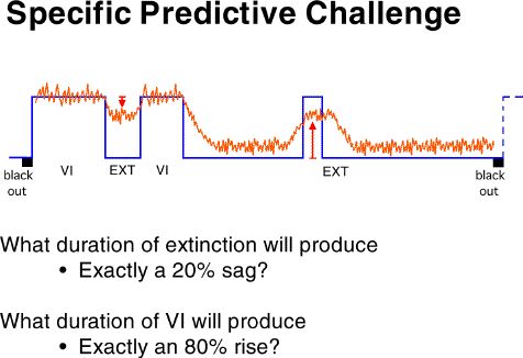
was then used to do two things: (1) generate the durations of the
VI schedules and the extinctions which would produce exactly a 20% sag
and exactly an 80% elevation in response rate for that particular bird,
and (2) generate an exact predicted output for that bird for each point
in time for that three-pulse procedure.
Our current solution is to no longer allocate so much of the spectrum
to behaviorally impossible frequencies. We are no longer sampling
at an extremely high rate which "detects" substantial amounts of high frequency
noise and then subsequently removes that noise with complex numerical methods.
By analogy, rather than measuring the time of pecks to the picosecond (which
results in substantial artifactual variability in the peck items) and then
smoothing down to milliseconds, we are measuring peck times to the nearest
millisecond. For example, it is simply not meaningful to emphasize
picosecond variability if pecks were to occur exactly 38 milliseconds apart.
The following is the obtained output for the test bird on the three-pulse procedure and the behavior predicted by the transfer function.
Obtained:
Predicted:
The important characteristics to note are:
While the transfer function predicts extinction "below zero," our procedure
was not capable of substantiating its existence.
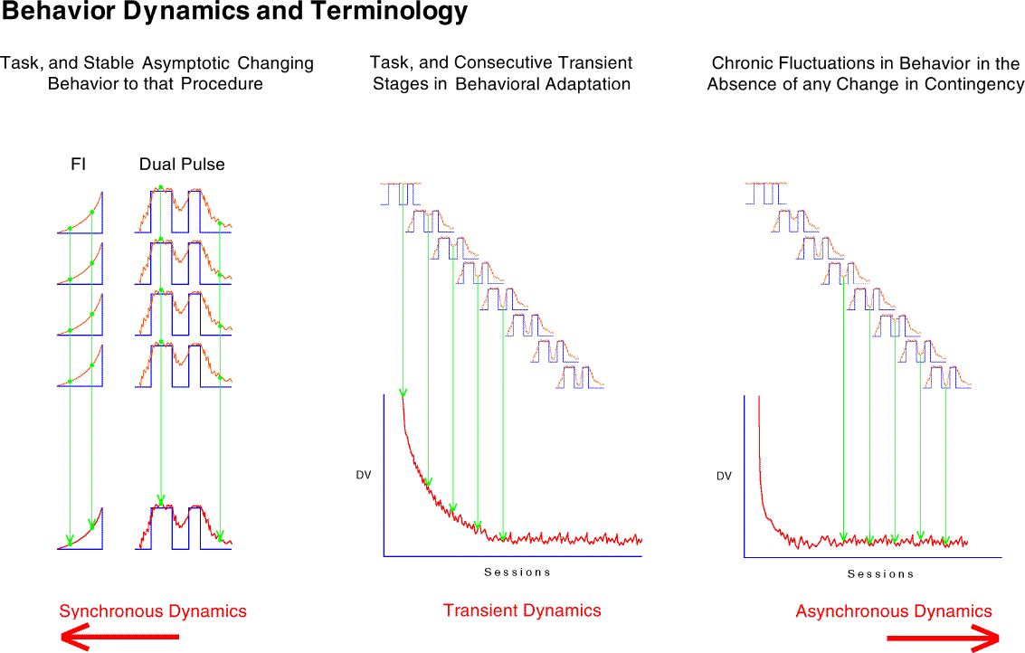
Transient dynamics are well known as "behavioral adaptation" or "the learning curve." These are not synchronous in that the function is a one time change.
Finally, the most poorly understood behavior dynamics are asynchronous dynamics. These changes are sometimes referred to as random unsystematic fluctuations in what is otherwise stable behavior. The grand challenge is to change as much of this residual variance to "variance accounted for" as is possible.
A detailed analysis of synchronous dynamics was presented by Palya (1992) in Dynamics and the Fine Structure of Behavior. The animated figure below illustrates the asynchronous dynamics in our two-pulse procedure for bird 568 from session 3 to session 192. Each of the 38 frames is the average of 5 sessions.