

 Figure 14
There are other factors which appear to vary the magnitude of the bitonic effect. They are therefore a good starting place for a functional analysis. The within-session effect appears to differ as a function of schedule of reinforcement. The left frame illustrates behavior under a VI while the right frame illustrates behavior under a VR with a somewhat similar reinforcement rate.
Additionally, reinforcement rate has been shown to have an effect on the within-session rate change. These two frames illustrate the strong effect associated with changes in reinforcement rate.
So, we explored the effect of 3 schedules and 5 reinforcement rates on the within-session effects with 12 pigeons. Each animal was exposed to each of the 15 procedures. The schedules were a VR with a VI+ and VI yoked to the reinforcement rate of the VR schedule. Each was implemented at the 5 reinforcement rates shown.
Note that the VI' schedules are yoked to the VR reinforcement rate. A VI'400 is approximately a VI 200.
Linear slopes were fit in the same way as in Experiment 1. An ANOVA (11 subjects * 3 schedules * 5 reinforcement rates) was nonsignificant. There was substantial noise. The medians are given in the table. The three-dimensional bars to the right provide the inverted data in order to provide a visual representation of the data surface.
If a rising and falling processes are at work across the session, then the conceptually simplest analysis is a two straight line fit.
This slide depicts the analytical procedure. The response rate in each 20-sec bin over the last 5 sessions was determined. The data were smoothed and then iteratively partitioned at each possible bin boundary. Two best fit lines were determined at each step. The set with the least residual variance was taken as the best two line fit. Error was then recalculated with the unsmoothed data.
The information obtained and displayed from the two line fits is depicted in this slide. The initial slopes are normalized to the last data point in each line. Similarly the second slopes are normalized to the first data point. Slope differences are presented as histograms. The breakpoints are presented as bars because of a systematic change with reinforcement rate.
This figure depicts the initial slopes for the 12 birds across the 15 procedures combined. The diagonal red line depicts the median slope. The histogram provides the distribution of slopes. The distance from the vertical green line to the normalization point depicts the length of the median first segment. It is the normalization point minus the median breakpoint.
This slide depicts the second slope across all birds and procedures. The red line again depicts the median slope. The histogram shows that there was relatively little variance around the typical second segment slope.
The table and figure shows that the median breakpoints typically occurred relatively early in the session and that they tended to occur later with decreases in the reinforcement rate.
This figure depicts the slope difference in the two slopes and shows that most typically, there was a greater deceleration or a lesser acceleration in responding or a lesser acceleration in responding from the first to the second slope.
This is the idealized distribution. It is constructed from the median initial slope, the median breakpoint, and the median second slope.
After documenting what did in fact happen as the result of changes in the schedule and reinforcement rate, the next obvious step is to determine the most appropriate model for that within-session rate change. Four models were examined: 1 straight line, 2 straight lines, McSweeney and Killeen. Each model was fit to the within-session rate change for each of the 12 birds under each of the 15 procedures. The reduced chi-squared for each model for each procedure is reported as a column of dots for each schedule. Lower numbers are better fits. The values are analogous to residual variance in a Pearson's r.
The 4 frames represent the fits made by the 4 models. The 15 columns in each frame denote the 15 procedures.
The 12 dots in each column depict the quality of fit for the 12 birds under that condition.
As can be seen, the simple straight line does nearly as well as the other fits and that the two straight does approximately the best. All 4 models do the worst with the VI behavior across the session.
The basic point is that a straight line function is fit equally well by all four models.
Experiment 2 Discussion
So, the take-home for Experiment 2: Overall there was consistency with McSweeney; typically, there was an increase in rate followed by a protracted rate loss throughout the rest of the session. However, in the present case, the magnitude of the effect was much reduced. The difference between our results and McSweeney's may have been her running procedure. She typically uses fixed session lengths and temporal termination, while our typical procedure is to run animals only long enough to maintain their body weight. Additionally, we terminate the session at the end of a reinforcer.

Date Last Reviewed : January 6, 2002
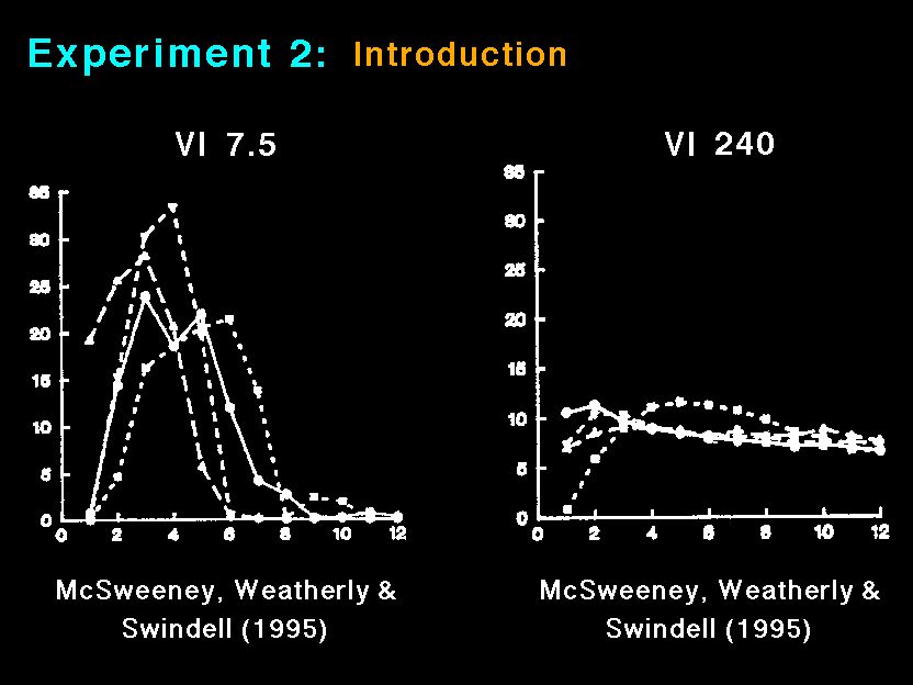 Figure 15
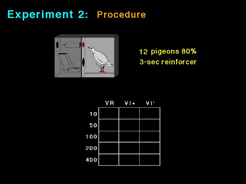 Figure 16
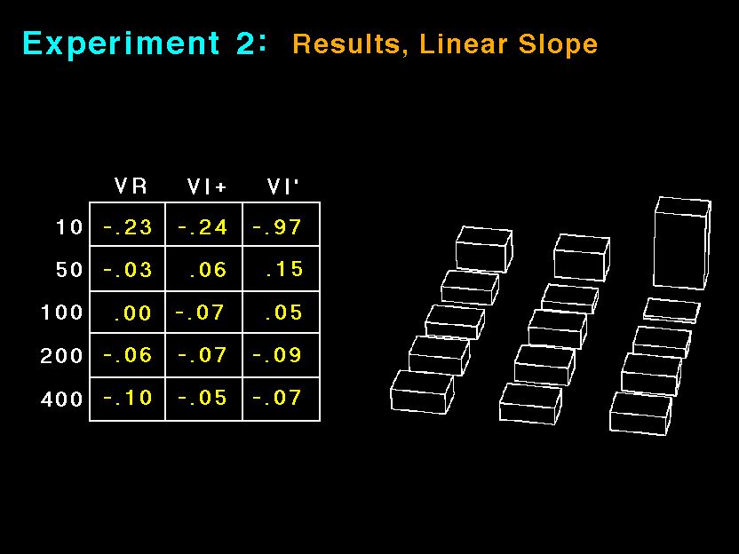 Figure 17
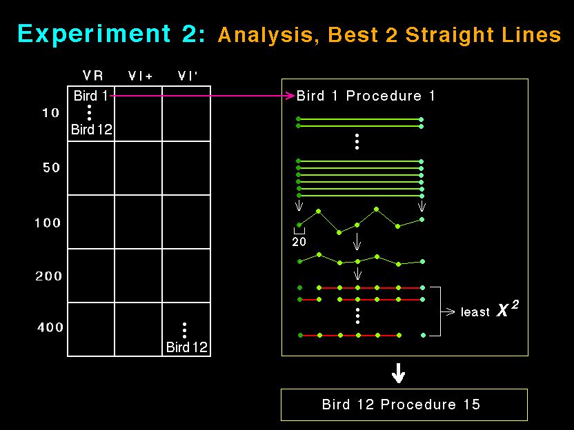 Figure 18
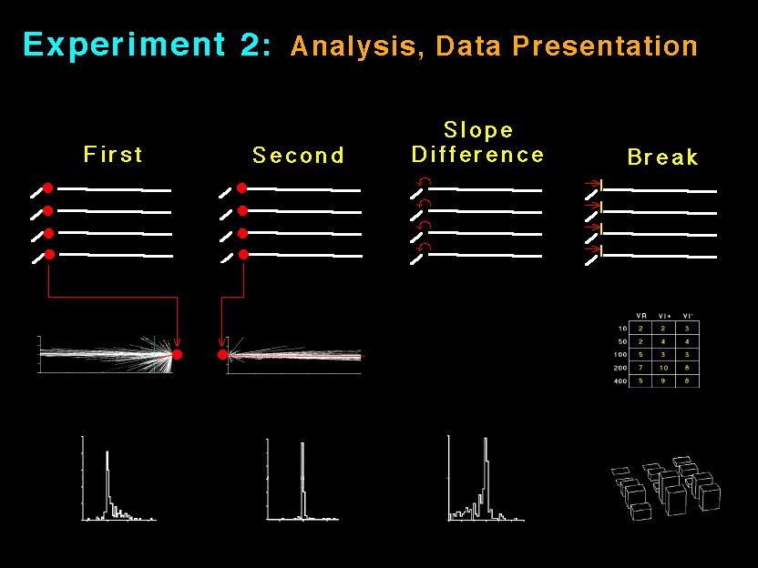 Figure 19
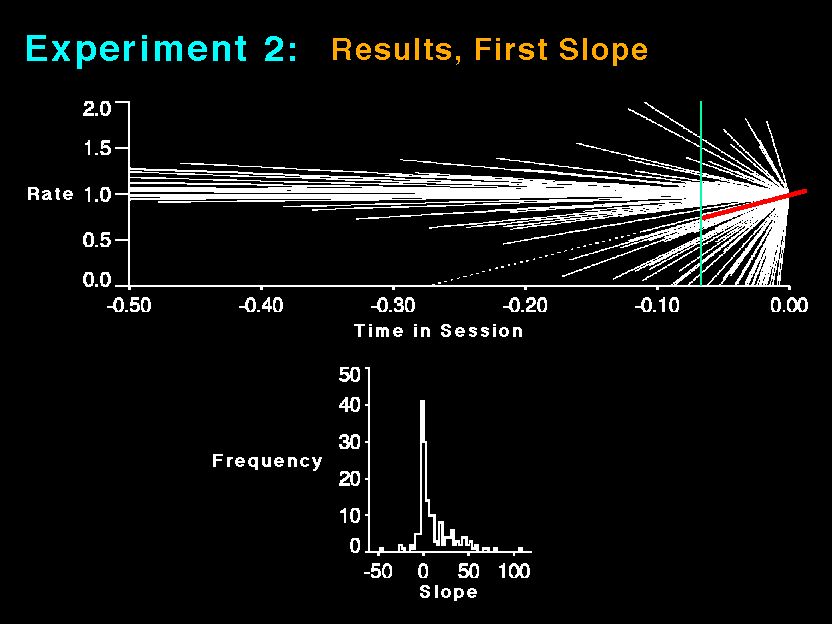 Figure 20
 Figure 20a
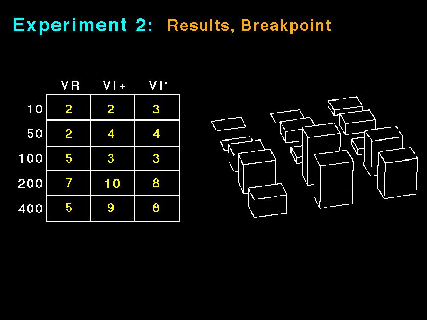 Figure 21
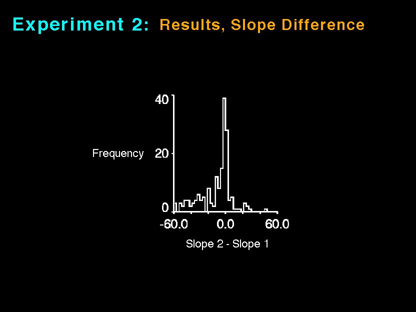 Figure 22
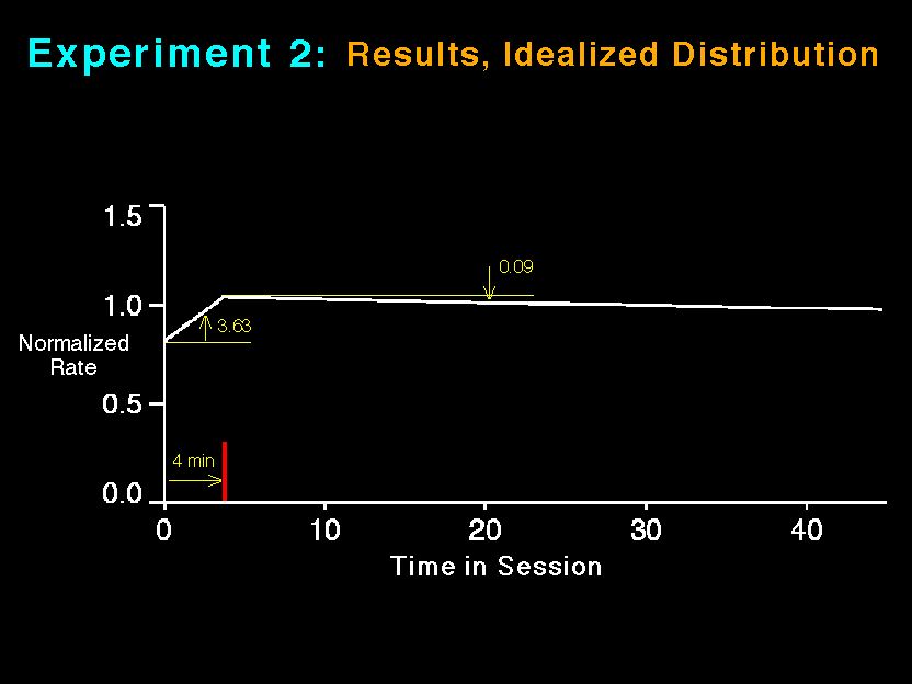 Figure 23
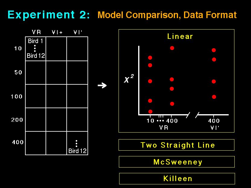 Figure 24
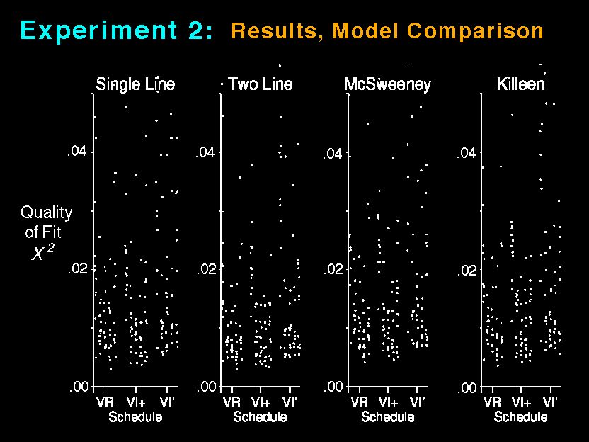 Figure 25
 Figure 26