
Jacksonville State University, Jacksonville, Alabama
Key words: dynamics, variability, chronic exposure, structure, automatic, interresponse time, sequential organization, key peck, pigeons
A slide/tutorial version of this paper is available at: The Fine Structure of Behavior
Psychology may be seen as the explanation of behavior change. The origin of that change is, therefore, at the heart of the science. Contingencies of reinforcement are used to good effect to explain the distribution of behavior between two simultaneously or consecutively presented schedules (Davison & McCarthy, 1988; Herrnstein, 1970), to a lesser effect to explain the distribution within a fixed temporal interval (Gibbon, 1977; Palya, 1985), and to poor effect to explain the various changes in behavior that continue to occur even after extended exposure to unchanging conditions (Zeiler, 1979).
Three general styles of explanation for chronic variability have been advanced: overcompensating homeostatic processes such as response strength mechanisms ( Herrnstein & Morse, 1958) or stimulus control mechanisms (Ferster & Skinner, 1957), external perturbations or noise (Sidman, 1960), and intrinsic variability. But precisely why homeostatic mechanisms fail eventually to dampen is left unexplained, and how what in truth are typically small amounts of random noise can overpower what are generally very strong schedule effects also remains unexplained. Finally, the postulation of an intrinsic cause for a phenomenon fails to provide a very useful explanation.
The emergence of an analytical paradigm based on nonlinear dynamics or chaos (Gleick, 1987) has provided a fourth alternative. Chaotic processes are simple deterministic systems that show continual, apparently random variation, much like the anomalous variability seen in operants maintained under steady-state conditions. It is interesting to note that Zeiler's (1979) characterization of the chronic variability in interval schedules--"the number of responses per reinforcement is highly variable, but it does not seem to follow a totally random pattern" (p. 113)--is remarkably similar to the subsequent descriptions of chaotic processes advanced by researchers in a wide variety of disciplines.
The present paper characterizes the chronic variability in behavior maintained under some "simple" contingencies of reinforcement. The behavioral variability in individual pigeons is depicted across various temporal windows. The paradigmatic perspective is that exposure to a contingency establishes a dynamic rather than a static behavioral equilibrium (Zeiler, 1979). The goal of the research is to document better the dynamic nature of that equilibrium. Birds were chronically exposed to the contingencies in order to obtain reliable estimates of the variability, to determine the degree to which the dynamics changed with extended exposure, and to provide a data base large enough to make any chaotic pattern in the dynamics apparent.
METHOD
Subjects
Six adult, experimentally naive White Carneau pigeons obtained from a local supplied were used. They were housed under constant illumination in individual cages with free access to water. All were maintained at approximately 80% of their free-feeding weights with pelletized laying mash.
Apparatus
Three experimental chambers were used. The interior of each was a 30-cm cube painted white. A stimulus panel served as one wall of the chamber. It had a feeder aperture 5 cm in diameter, medially located 8 cm above the grid floor. Three response keys, 2 cm in diameter, were located 9 cm apart, 19 cm above the grid floor. They required approximately 0.15 N to operate and had 30-ms debounce times. Only the center key was used. The translucent Plexiglas key could be transilluminated yellow-green by a stimulus projector containing a Rosco (#878) theatrical gel. Two houselights were located 28 cm above the grid floor and 9 cm apart. Ventilation was provided by an exhaust fan mounted on the outside of the chamber. A white noise generator in each chamber, as well as in the room itself, provided ambient masking noise. The houselights and keylight were off and the magazine light was on during food presentation. Each session typically contained 40 food presentations, as determined by the bird's body weight that day. Stimulus events were controlled and key pecks were recorded by a computer system (Walter & Palya, 1984) .
Procedure
The effects of chronic exposure to a schedule of reinforcement on the dynamics of operant key pecking were observed with 6 pigeons. Each of six basic schedules was implemented with a different bird. Each bird was exposed to those procedures daily. The present results included data across 780 sessions of exposure to the same contingencies. The schedules were: fixed-interval 60 s (FI 60); fixed-ratio 60 (FR 60); variable-interval 60 s (VI 60); variable-ratio 150 (VR 150); differential reinforcement of high rate, implemented as a VR 80 composed entirely of IRTs less than 0.8 s (any IRT exceeding the criterion reset the ratio; DRH 80/0.8); and differential reinforcement of low rate 20 s (DRL 20).
Following magazine training and manual key-peck shaping, the schedules were adjusted over the course of several weeks to the above values so that each schedule provided approximately 60 reinforcers per hour. The DRH schedule was initially implemented as a DRH 80/0.4. After 90 sessions it was changed to a DRH 80/0.8. The DRL was initially implemented as a DRL 15 schedule. After 60 sessions it was changed to a DRL 20 schedule. The FR was initially implemented as an FR 75. After 60 sessions, it was reduced to an FR 70; after 30 more sessions, it was further reduced to an FR 60. The variable schedules were initially based on exponential values ( Fleshler & Hoffman, 1962). After 150 sessions the distributions of values underlying the VI, VR, and DRH were changed to rectangular distributions of values. Following approximately 200 additional sessions, these schedules were returned to exponential distributions. Only the sessions following stability under the final schedule parameters were included in the summary presentations. The performance maintained by the DRH schedule began to deteriorate after about a year's exposure to the schedule. Compensatory changes in schedule requirements negated the usefulness of the subsequent data to characterize variability independent of schedule changes.
Complete interevent time records, to the nearest millisecond, were obtained and stored by the experiment-control computer network. Each stimulus and response event was recorded with respect to its time of occurrence and was permanently archived. Data analyses were subsequently carried out on these archived interevent times.
RESULTS
The results were grouped with respect to schedule, measure, and temporal window. The schedules were the six basic contingencies presented in the procedure section. The measures were the preresponse pause (PRP) or the pause preceding the first response in each interreinforcement interval (IRI), the mean rate of responding in each IRI, and the relative frequency of each interresponse time (IRT). The temporal windows ranged across the entire period of exposure to the contingencies, across a session, and across the IRI. These windows document, to use a broad interpretation of Skinner's (1938) terminology, deviations of the first, second, and third order, respectively. Because of the importance of characterizing the variability within a bird's behavior, the axes' scales were a compromise between providing for an immediately apparent comparison of schedules and most clearly illustrating the variability within a frame.
Preresponse Pause Measure
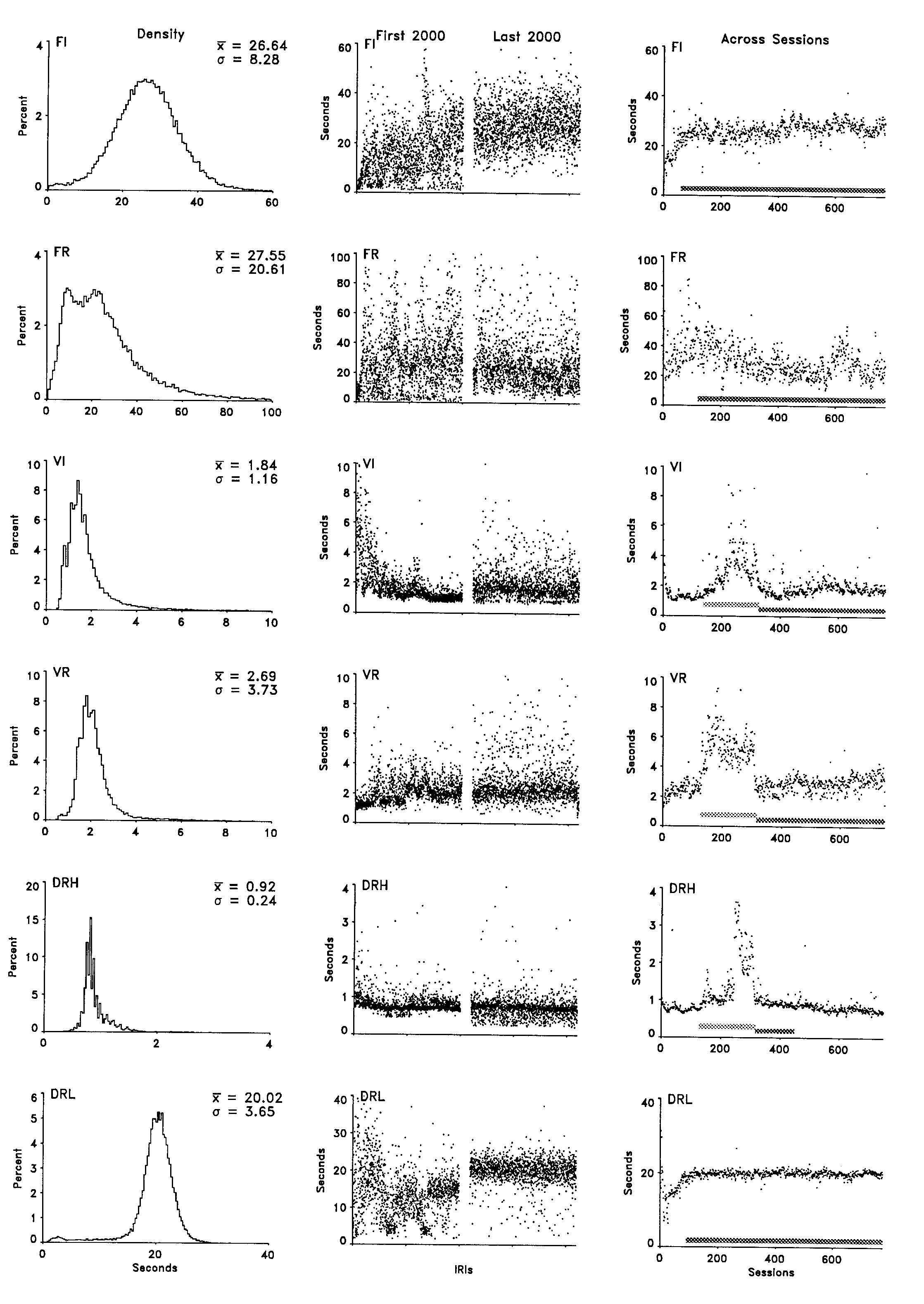
The center column of Figure 1 depicts, for each of the indicated schedules, the duration of the pause preceding the first response in each of the initial 2,000 consecutive IRIs (left portion) and each of 2,000 consecutive IRIs following extensive experience (right portion). These data were taken from the earliest and latest sessions depicted in the right-most frame. Each half of the frame shows the data for each trial over the course of approximately 50 sessions. Consecutive IRIs are depicted across the x axis. Pause length is depicted on the y axis. (Note that the x axis is compressed.) The data are depicted with no lines connecting the consecutive points so that the visual weight of the figure is carried by the data rather than by the lines connecting those data. Because the 2,000 consecutive PRPs extended across multiple sessions, any systematic changes in the PRP across a session would contribute to this depiction of variability. However, these effects do not contribute to the apparent cyclicities shown in these frames in that the x-axis extent of each session is only approximately two dot diameters wide. As noted in the procedure section, some schedules were changed across the initial sessions of exposure to adjust the reinforcement rate. As a result, the first 2,000 IRIs for the FR, DRH, and DRL, birds portray both a schedule effect and a learning effect, as well as residual variability.
The variability in the PRP showed some changes across the approximately 700 sessions that intervened between the data shown in the left and right portions of each frame; however, there was surprisingly little decrease in the variability considering the amount of experience separating those windows. In general, the frequency of short pauses decreased under the FI contingency, and the variability in the pause preceding the first response actually increased under the VI and VR contingency. The DRL schedule produced a very stable pattern of initial pauses, which was apparent in both this column and the right-most column. The changes in behavior under the DRH schedule illustrated in this frame include those that occurred as a result of the schedule adjustments.
The right column in Figure 1 portrays the mean seconds of pause preceding the first response for each of the 780 consecutive sessions with a point. Mean seconds of pause for a session is depicted on the y axis, and consecutive sessions are depicted across the x axis. The most obvious effect across exposure to the procedure was the increase in the PRP associated with the change from an exponential to a rectangular distribution of values in the variable schedules. This procedural change is indicated with a marker along the x axis (the upper one). This schedule-dependent effect was not the focus of the present paper, and none of the comparisons included these data. The changes in the left-most portion of each of these frames were also outside the scope of the paper. Those changes documented the initial behavioral adjustments to the schedules and the changing contingencies. Of present interest are the residual variability in the session-to-session averages, the slow oscillations, and the systematic trends across the course of the experiment. The clearest trend was apparent in the final portion of the DRH schedule. It documented the slow collapse of the behavior noted earlier. It included the schedule adjustments across the same period and was therefore not especially informative. The slow decrease and subsequent transient increase in the PRP under the constant FR schedule was notable, but is presently inexplicable. The session-to-session variability in the PRP increased under the exponential schedules, but otherwise was generally constant across most of the exposure to the contingencies. The PRP under the FR schedule exhibited the greatest reduction in variability, but that was confined to the first 200 or so sessions.
Rate Measure
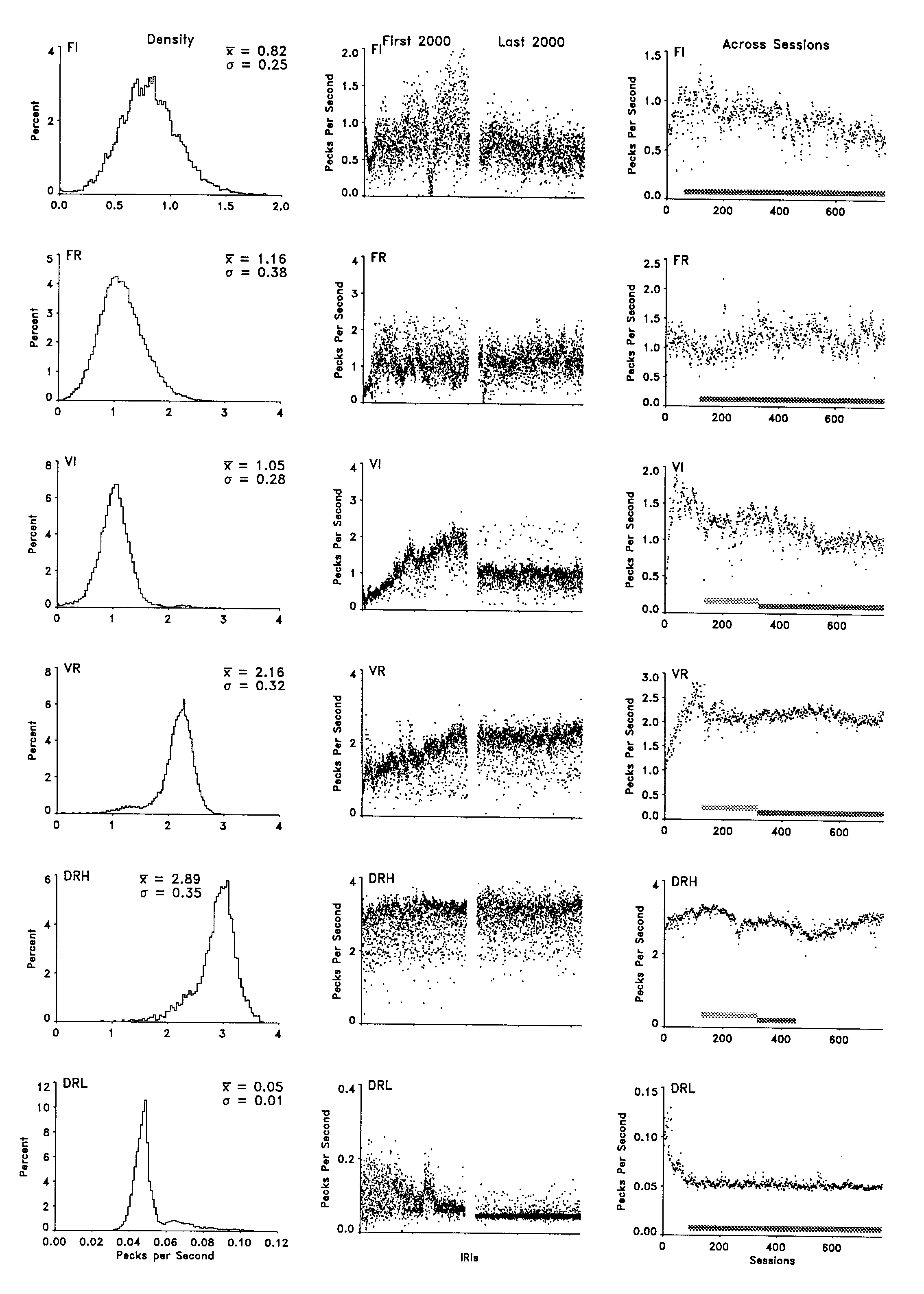
The changes in the mean response rate in each of the initial 2,000 IRIs and the final 2,000 IRIs are depicted in the center column of Figure 2. Although mean rate changed in several cases, substantial reductions in variability did not occur over the approximately 700 session separation between the windows. The clearest decrease in variability was exhibited by the DRL schedule. The response rates under the FI schedule also showed some reduction in variability. The change in the FI rates occurred mostly as the result of a decrease in the frequency of higher mean rates. Slow, somewhat periodic oscillations, similar to those used to describe response count variations in FI schedules by Dews ("irregular periodicity that was seen as a waxing and waning of the prevailing numbers of responses m sequences of intervals"; 1970, p. 59), occurred under the FI and FR schedules and to a lesser extent under the initial exposure to the VI schedule.
The right column of Figure 2 shows the changes in the mean rate for each consecutive session. The rectangular distribution of values for the variable schedules had a surprisingly small effect on the rate measure considering the change in the amount of the interval occupied by the PRP. The FI and VI schedules controlled a general decrease in rate across exposure to the schedules. FI rates showed the largest decrement, but that was confined to the first 100 or so sessions. There was an increase in the FR rate, consistent with the decrease in the PRP for that bird shown in Figure 1. Responding under the DRL schedule showed a substantial initial decrease in rate followed by stable rates throughout the remainder of the experiment. In general, the variability in the mean session rate, from session to session across the entire experiment, showed little change, similar to the PRP measure.
Session Window
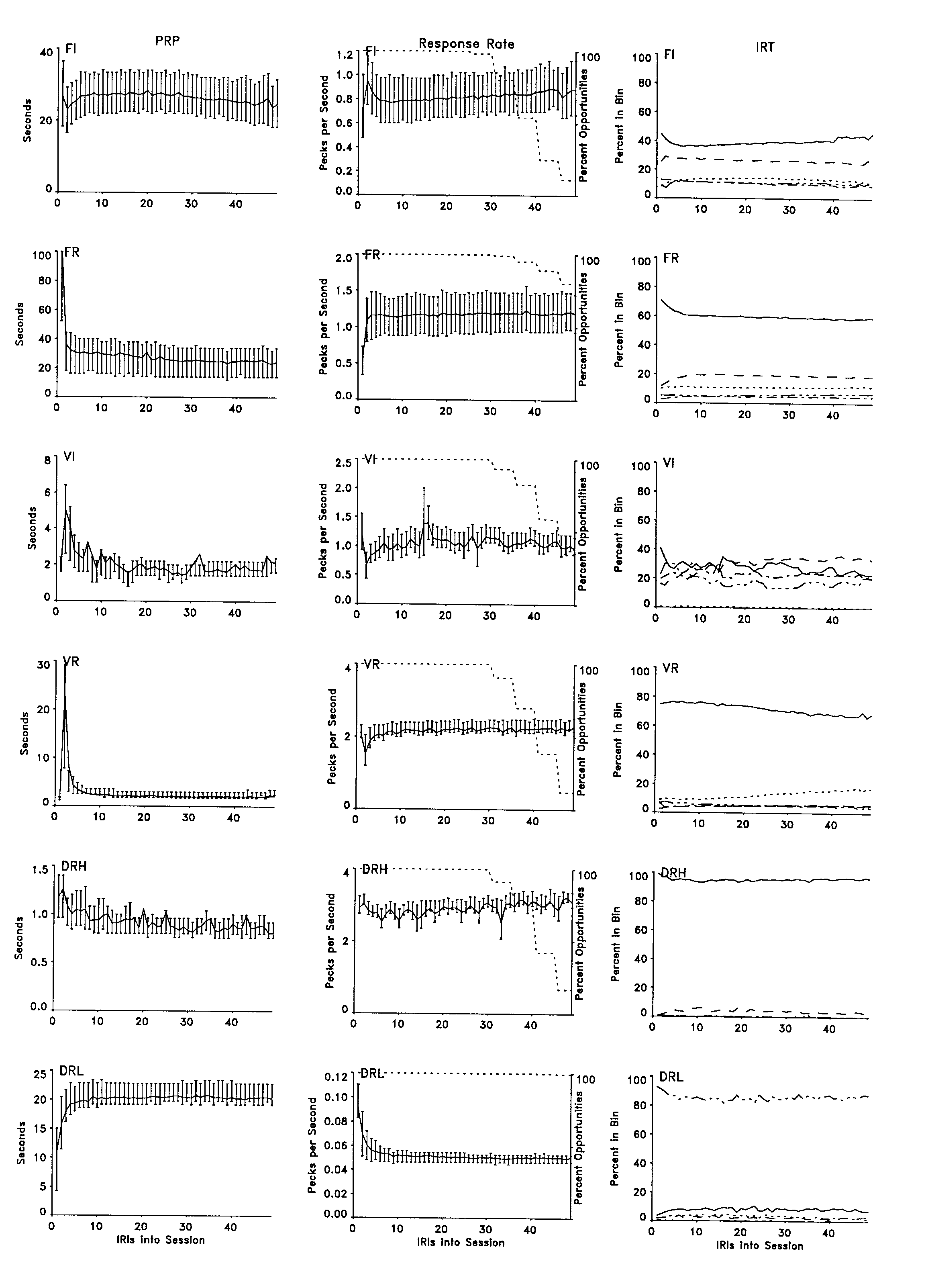
The left column in Figure 3 depicts changes in the mean pause before the first response, for each consecutive IRI in a session. The y axis designates seconds of pause, and the x axis indicates ordinal position in the session. The first data point in each frame indicates the time from session start to the first response. With the exception of the first few IRIs, mean PRP and the quartiles of the distribution for the PRPs in each ordinal position remained relatively constant throughout the session. The FR, VR, and DRL schedules controlled the greatest change across the first few IRIs, and the pauses under the DRH and FI schedules showed the least. The changes in the PRP across the session under the DRL schedule were consequential. Early in the session most PRPs fell well below the DRL requirement, but later in the session most PRPs approximated the 20-s IRT requirement. The premature responding (the bulk of the IRTs between 5 s and 15 s) can also be seen in the frame depicting the distribution of IRTs across the IRI for the DRL schedule (Figure 4) as well as in the subsequent frames depicting individual IRTs.
Changes in the mean response rate for each IRI across the consecutive IRIs of a session are depicted in the center column of Figure 3. The y axis designates response rate, and the x axis indicates ordinal position in the session. The FI and DRH schedules controlled a slight increase in rate across the session. Otherwise, most schedules controlled relatively similar mean rates and distributions of rates across the entire session, with the exception of the first few IRIs. These frames present a picture similar to those depicting PRP and lend support to the practice of excluding the data from the first few IRIs of a session when calculating summary statistics intended to represent typical performance.
(A slide version of some of this IRT information is available).
The right column of Figure 3 presents the relative proportions of IRTs in each of five bins across the consecutive IRIs in a session. The y axis specifies the proportion of IRTs in each bin, and the x axis depicts position in the session. The bin boundaries are selected individually for each bird and can be most easily specified by reference to Figure 5. The solid line depicts the band of IRTs that centers at approximately 0.35 s (the "main band") and extends for half its period in either direction. The first and second subharmonics of this band (e.g., at 0.7 s and 1.05 s) are designated with a dash and a dot-dash, respectively, whereas all longer IRTs are represented with a triple dot-dash. All IRTs below the main band are represented with a dotted line. Behavior under the FR, VR, and DRH schedules showed a clear preponderance of responding at the main band, whereas the FI and VI schedules controlled a more even distribution of IRTs across the various bands. Behavior controlled by the DRL schedule showed responding in the band at approximately 0.35 s, but, as would be expected, most IRTs were above the first two subharmonics of that band (at the required IRT of 20 s). In general, all schedules maintained very stable distributions throughout the session following an initial adjustment at the beginning of the session. There were two exceptions. The IRT distribution maintained under the VR schedule showed a systematic change in the proportion of responding in the main band and in the bin of shorter IRTs. Although this change was small with respect to the difference in the amount of behavior occurring in those bands, it was a trend across the entire session. The second consistent change across a session can be seen in the behavior maintained by the VI schedule. This schedule controlled a slight decrease in the proportion of responding in the main band and an increase in the first subharmonic (IRTs centering at approximately 0.7 s) as the session elapsed.
Interreinforcement Interval Window

The left column of Figure 4 depicts the probability of a PRP extending to each point in the IRI. It provides the same information in a different format as that presented in the left column of Figure 1. Roughly half of the PRPs in the FI schedule were terminated before the midpoint of the interval, and half of the PRPs in the DRL schedule were terminated before the DRL requirement. The VI, VR, and DRH schedules rarely generated long pauses. The PRP under the DRH schedule exceeded a few seconds less than 1% of the time, whereas the PRP under the VR schedule extended as much as 30 s in 2% of the IRIs. Analysis of the VR pausing indicated that most of the PRPs in excess of a few seconds occurred in the first few IRIs of a session. This can be seen in the frame depicting PRPs for the VR schedule across the session (Figure 3).
The center column of Figure 4 depicts the mean response rate at each point in the IRI. The degree to which these changes in the mean rate actually reflect changes in the momentary rate, rather than simply the probability of responding, is best assessed by comparing these rate data with the distribution of PRPs in the left column, the IRT data in the right column, and the IRT data presented in Figure 5. The center column of Figure 4 shows that behavior under the FI and FR schedules exhibited an increasing mean rate, followed by a subsequent decrease, whereas the VI, VR, and DRH schedules controlled an initial sharp increase in mean rate followed by a somewhat constant mean rate throughout the remainder of the IRI. The responding in the DRL schedule exhibited a cyclic mean rate change with a 20-s period.
The right column of Figure 4 shows changes in the IRT distribution across the IRI for each schedule. The y axis designates the proportion of responding in each bin, and the x axis designates consecutive portions of the IRI. The IRT bin represented by each function is the same as that used in Figure 3 and is directly comparable to the frames in Figure 5. Although this column presents the proportion of pecks at each IRT value at each point in the IRI, Figure 5 presents the IRTs themselves at each point in the IRI. This column can be seen as a summary of the data in Figure 5; alternatively, Figure 5 can be seen as providing the variance information for these frames. With the exception of the first few seconds of the IRI, the distribution of IRTs across the IRI indicated that the IRT distribution was relatively stable from reinforcer to reinforcer. The FI schedule showed the most notable exception. There was a change in the dominant IRT during the final quarter of the interval. The impact of this change on the mean rate was apparent in the rate frame for this bird immediately to the left and can be seen in the IRT-IRI frame for this bird in Figure 5. A second notable exception was apparent in the frame depicting the behavior under the DRL schedule. The spike in the function designating the proportion of long IRTs (the triple dot-dash line) between 5 s and 15 s was primarily due to IRTs in that range that occurred only early in a session. Otherwise, this line for the most part depicts IRTs of approximately 20 s; those, of necessity, could not begin until 20 s into the interval.

There was a striking regularity in responding, both across the IRI and across schedules and birds. There was a clear preponderance of IRTs around particular unchanging values, with fewer IRTs of intermediate value. In each case, a prominent band occurred at approximately 0.35 s. In the case of the schedules other than DRL, there were additional bands at integer multiples of that base time (e.g., at 0.7 s and 1.05 s). This characterization was especially appropriate in the case of the DRH schedule but was less appropriate for the Vl schedule, which controlled many IRTs of intermediate value. The means and variances of the bands remained relatively constant across the IRI. The general characteristics typically applied to schedule-controlled behavior can also be seen in these frames. Behavior under both the FI and FR schedules exhibited a general absence of responding in the initial portion of the IRI, whereas both the Vl and VR schedules showed an immediate onset of responding. Both interval schedules also controlled more responding at subharmonics of the main band than did the ratio schedules. This pattern of behavior resulted in lower running rates in the interval schedules. These characteristics had been discernible from virtually the onset of consistent responding, and exhibited very little change across the remainder of the experiment.
One aspect of the data in these frames appeared to be idiosyncrasies of individual birds. The occurrence of IRTs shorter than the main band showed substantial bird-to-bird variability. (This interpretation is supported by comparison with data obtained from other birds under similar procedures in this laboratory.) In the present case, the FR and VR frames showed a diffuse band, Fl showed two thin distinct bands, and Vl and DRH showed virtually no responding below the main band. The behavior in this class of IRTs was evaluated with other birds in order to determine whether it was caused by multiple outputs from a key attributable to the mechanical properties of the key itself (e.g., key bounce). It occurred with "snap action" switches (e.g., Lehigh Valley keys), lever arm switches with only normally closed contacts (e.g., Gerbrands keys), and specially designed lever arm switches that required the "break" of a normally closed contact followed by the "make" of a normally open contact. In addition, various idiosyncratic properties of the band of very short IRTs were robust across changes in the force requirement and throw distance of the keys.
The lower right frame of Figure 5 depicts IRTs as a function of time in the IRI under the DRL schedule. Some of the behavioral dynamics portrayed in this frame occurred on a different time scale than in the preceding frames, and their interpretation benefits from additional explanation. As with the other IRT*IRI figures, the termination of food presentation is represented at the origin. The first-peck line can clearly be seen in the left portion of the frame. If an IRT exceeded 20 s, it was followed by food and the next response was again timed from the origin. Otherwise, the ordinate was reset to zero while the abscissa continued to increment, much like the resetting of a cumulative recorder. Approximately half of the first pecks in the IRI failed to exceed the 20-s criterion. As time in the IRI continued to elapse following the first response, the x,y position appropriate for the depiction of the next peck was incremented at the diagonal set by the axis ratio. If another unreinforced response occurred, the y position was again reset to zero while the x axis continued to increment. As long as responses failed to meet the requirement for reinforcement, this sawtooth pattern was repeated for each response.
This graphical procedure produced diagonal clusters at the subharmonics of the DRL requirement and clearly illustrated the distribution of IRTs around the 20-s requirement, as well as depicting the distribution of IRTs as a function of time since the reinforcer. The variance along the first-peck line was attributable to the variance in the time of the first peck. Nonreinforced first pecks reset the IRT. time to the x axis. If second pecks occurred immediately, the variation in the latency to the first response created the horizontal variance in the cluster along the x axis, especially noticeable between 15 and 20 s. The variance perpendicular to the diagonal loci of the second long IRTs was, for the most part, also attributable to the variance of the antecedent behavior. Variance along the diagonal, on the other hand, was attributable to the variance of the IRT that occurred at that subharmonic. The sharp edge to the right of the first subharmonic was attributable to the fact that none of the IRTs exceeding the 20-s DRL requirement continued incrementing across the x axis, but rather reset to the origin. The first subharmonic was, as a result, primarily composed of IRTs following the lower half of a normal distribution of first pecks centering on a 20-s latency to the first peck. Each successive subharmonic repeated this pattern.
Sequential Dependencies
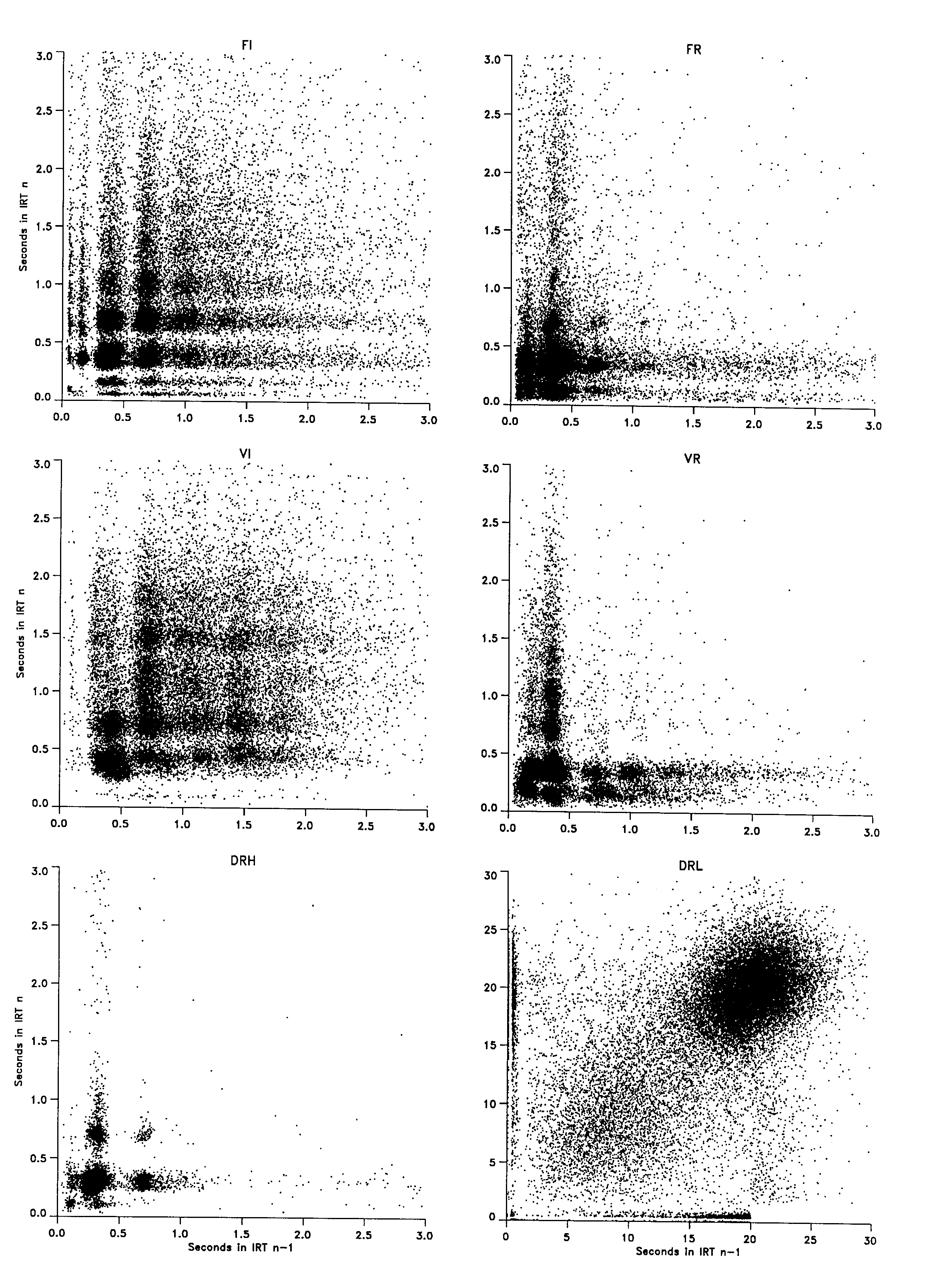
Each frame in Figure 6 may be seen as a graphical implementation of a contingency table. If the clusters or cell frequencies were not different from a joint function of the proportion of pecks in each band or marginal totals, then a sequential pattern was not demonstrated. With the exceptions noted below, the frames failed to show a sequential pattern in the obtained IRTs. The density of each IRTn * IRTn-1 cluster appeared to be simply proportional to the number of IRTs in the bands that formed that conjunction. Changes in the figure going from bottom to top were essentially the same as those going from left to right. There was symmetry around the main diagonal.
The most obvious asymmetries occurred under the DRL schedule and were the result of food presentation. The sharp edge in the lower right portion of the frame 20 s into the interval reflects the fact that if the prior IRT had been greater than 20 s, it was followed by food, and the next peck was unlikely to occur within the first second following removal of the food magazine (i.e., the peck following a reinforced peck is the first peck in the next interval). An additional insight into the distribution of IRTs following food presentation is provided by the distribution of PRPs in the lower left frame of Figure 1. Because PRP and the first IRT after food presentation are equivalent, the frame in Figure 1 depicts the density of various IRTs following all IRTs greater than 20 s. A second effect of food presentation on the DRL performance was that the distribution of IRTs following the reinforcer (>20 s on the x axis) was slightly skewed with respect to the distribution of IRTs following a preceding peck ( < 20 s on the x axis). This difference resulted in an apparent vertical split and upward displacement of the right portion of the large cluster of dots centered on the 20-s IRT requirement. This effect is dependent on the relative dot size and is especially apparent in large-format displays of this frame.
The second exception to the otherwise simple stochastic patterning in the various frames of Figure 6 occurred under the VR schedule. There was a discernible asymmetry in the cluster of responding at 0.15 s and 0.22 s. In that the sum of those two consecutive IRTs approximated the dominant main band IRT of 0.35 s, it appeared that a main band IRT was asymmetrically split into two shorter component IRTs. This would occur if the main IRT band were under the control of forward and backward head movements, while the asymmetrical split was generated by an upper and lower bill contact or by a key strike followed by a sideways head movement or "flick" that operated the key again but that did not change the period of the forward and backward head movement.
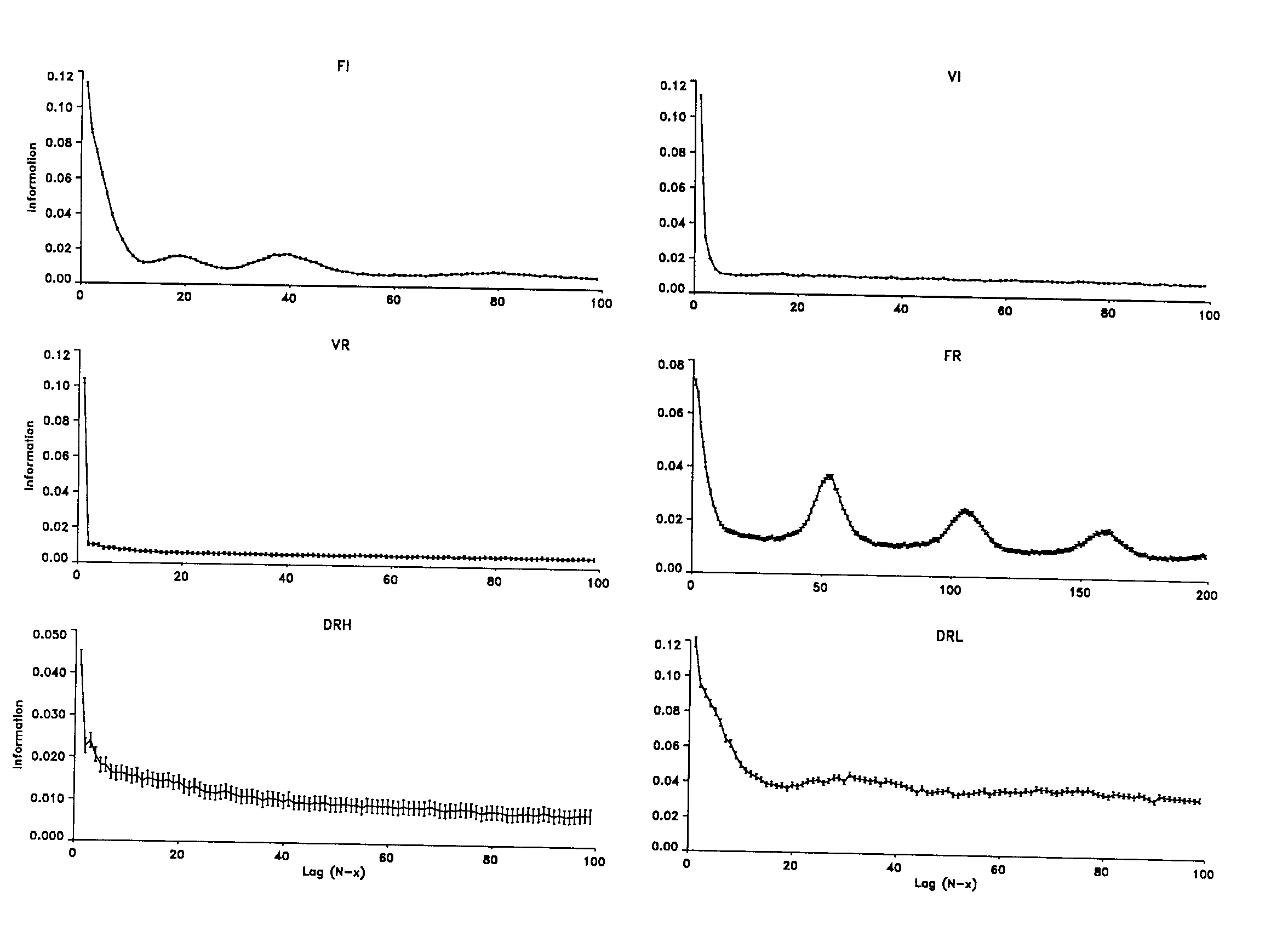
Although there was no sequential ordering to the IRTs systematic enough to be apparent in the IRTn * lRTn-1 figures, it is possible that some more powerful quantitative index could identify one. This would be the case especially if that index were sensitive to sequential dependencies across lags greater than one. Figure 7 depicts the extent to which any particular IRT duration can predict some subsequent IRT duration. This figure provides the "information stored" or "information carried forward" (Shannon & Weaver, 1962) in temporally successive distributions of IRTs . Information in this context is the degree to which the distribution of IRTs following an IRT in one particular bin was different from the distribution of IRTs following an IRT of some other value. The effect could be immediate, in the sense that an IRT may affect only the distribution of the next consecutive IRT, or the effect could occur only after some number of intervening responses. The information would be zero if the IRT distribution were the same regardless of the prior IRT or if the variation were random. Potential information would increase as the number of alternatives increased. For example, prediction in the context of two possibilities would be one bit of information, whereas prediction in the context of four possibilities would be two bits. The stored information in the last 300,000 IRTs from 0.2 s to 3.0 s for each schedule (the last 50,000 IRTs from 10 s to 30 s in the case of DRL) was therefore determined and is presented in Figure 7. Because of the sample size, this index is capable of identifying sequential dependencies of a magnitude not readily apparent in an IRTn * IRTn-1 display. IRTs below 0.2 s were excluded in order to remove as much of the sequential information in upper and lower beak hits from the measure as was practical with an arbitrary criterion. The IRTs above 3.0 s were excluded so that the obtained indices would apply to the same data as were depicted in Figure 6. Because of this data selection criterion, the analysis targeted sequential dependencies at a level below that attributable to long pauses followed by responding such as that exemplified by responding under an FI schedule. The DRL window was selected in order to examine the sequential dependencies in the IRTs centering on the DRL requirement. This provided the information in behavior appropriate to the schedule (i.e., IRTs ~ 20 S) at the expense of also indexing the information provided by the tendency for many of those IRTs to be followed by an IRT of approximately 0.35 s. The whiskers at each data point depict the uncertainty in the measure at that point. The algorithm was derived from Shannon and Weaver (1962) by Shaw (1984) and was implemented by Kessel (Pevey, McDowell, & Kessel, in press).
As can be seen by noting the y axis scales in the various frames of Figure 7, there was little sequential information in the IRT distributions. However, by expanding the y-axis scale, the systematic changes in the sequential information and the decay to entropy in the sequential measure can be seen across the successive lags depicted in each figure. To the degree that it is reasonable to consider that any information or sequential dependency remaining after a lag of 100 was noise, then most schedules were stochastic within a lag of 10 responses. The information stored in all but the DRL schedule quickly dropped and asymptoted at just below 0.02 bits of information with increasing lags. In comparison, the same analysis carried out on the output of a logistics function ~(x) = 2.9x(1--x)] (Staddon & Ettinger, 1989, p. 118) had just less than 4 bits of stored information at a lag of I and 1.3 bits of information at asymptote.
Schedules with major events synchronized to a constant number of responses (e.g., FR, and to a lesser extent FI or even DRL) exhibited small (<0.02 bits) but reliable exceptions across increasing lags, at multiples of the number of responses in their respective IRIs. Because only IRTs between 0.2 s and 3.0 s were included in this analysis, changes involving the PRP did not contribute to this effect. Careful examination of behavior under the FR schedule showed a slight but consistent drop in the mean IRT in the main band across the first 10 or so responses in the ratio (as if the timing of the behavior were at least partly under the control of the motion involved, and the bird moved slightly closer to the key). In addition, the probability of a response with an IRT in the first, second, or third subharmonic increased across the last 10 or so responses in the ratio. The stored information exhibited by the behavior under the FI schedule showed a somewhat similar dynamic based on the response count. It appears that the increase at Lag 40 was attributable to a regularity correlated with the number of responses in the interval, whereas the peak at Lag 20 may have been attributable to the shift to longer IRTs than those in the main band following a run of about 20 responses, as previously noted. The DRL schedule showed the greatest degree of residual sequential dependency, with 0.12 bits of information decreasing to approximately 0.04 bits across 15 lags. In addition to any incommensurability caused by the necessary differences in the analysis parameters because of differences in the time scale of this behavior, the stored information in the behavior under the DRL schedule seems to be attributable to the sequential structure in the behavior that has been noted previously. In sum, all of the above stored-information findings have their greatest significance in demonstrating a relatively small upper bound on the sequential dependency in the behavior supported by these reinforcement schedules. There was no indication of strong sequential organization beyond the relative minor dependencies already apparent in the IRT-IRI and IRTn-I figures.
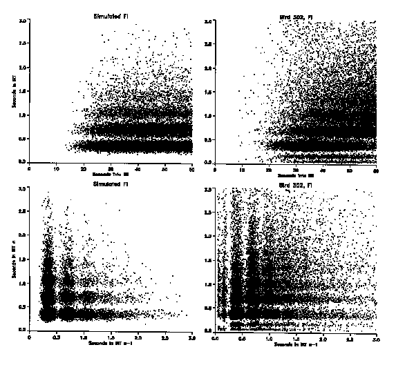
Output Simulator
In order to understand better the nature of the behavioral regularity underlying the patterns obtained in Figures 5 and 6, a pigeon was simulated with a computer algorithm. The goal was to reproduce the IRT*IRI and IRTn * IRTn-1 figures for the behavior obtained under the FI schedule. As a result, the simulator addressed the dynamics of the behavior at steady state but did not address the acquisition of that behavior. The simulator's basic element was a simple recurrent pulser. Observation of the birds had indicated recurrent movements, many of which occurred at the appropriate time but did not operate the key. These were not simply key contacts that failed to be recorded as a peck. Rather, they included very small movements toward the key when a movement of several centimeters would have been necessary, pecking motions directed away from the key, simple beak openings, and even body motions totally unlike key pecks but that occurred at the basic recurrent pulse time. The simulator's basic pulse time was set to 0.35 s (2.86 Hz) in order to coincide with the mean of the main band exhibited by the bird under the FI schedule. If plotted on the IRT-IRT frame, the simulator's simple pulse output would produce a horizontal row of dots across the entire frame 0.35 s apart and 0.35 s above the x axis.
The frequent, apparently random, absence of a peck at some pulse times was simulated by randomly deleting 35% of the pulses. This value was selected to match the actual output seen on the FI schedule. If plotted, the output of the model then would produce horizontal rows, one above the other, of dots across the width of the frame at integer multiples of 0.35 s above the x axis. Gaussian noise with a standard deviation of 0.05 s was added to each pulse in order to simulate variability and thereby produce the bands apparent in the output depicted in Figure 5, rather than simple rows of dots. Again the values were chosen to match roughly that which occurred under the FI schedule. The PRP for each IRI was selected from a Poisson distribution of times with a mean selected to match the obtained data (27 s). This function is consistent with previous work in this and other laboratories that has demonstrated that behavior under fixed intervals can be seen as the result of bipolar control that splits at roughly the midpoint of the interval. The initial half of the interval controls avoidance or escape, whereas the final portion controls approach ( Palya & Bevins, 1990).
DISCUSSION
The initial purpose of the present research was to characterize the dynamics or residual variability maintained by "simple" contingencies of reinforcement. An extensive archival data base on the variability chronically maintained by simple schedules was generated; the most notable finding was the clear recurrent responding at somewhat less than 3 H~ in every bird, even after extended exposure to the schedules and regardless of their individual contingencies. There did not appear to be any strong sequential dependencies in this recurrent responding, and no nonlinear dynamical descriptor for the band-to-band transitions was identified.
In spite of the considerable progress that has been made since 1938 in understanding the determinants of behavior change, the present results draw attention to several analytical traditions. The results indicated that there remain substantial changes in the mean value of some dependent measures even after hundreds of sessions of exposure to the contingencies. Simply taking the mean of 5 or 10 sessions at some point in the exposure would not necessarily have resulted in a "true score." This variability, in light of the increasing importance of detailed quantitative comparisons, argues for an examination of the criterion used to select commensurable measures of behavior. If both extended exposure and initial exposure produce erroneous five-session means, then the best window within which true scores can be obtained should be identified. Second, the session-to-session and trial-to-trial variability, irrespective of long-term shifts in the mean value, was sufficient to warrant more theoretical attention. The reliance on point estimates in the face of the demonstrated magnitude of pervasive chronic variation may not be the most productive technique.
As a minimum, determination of the appropriate characterization of the processes underlying that variability offers the opportunity for better prediction. The chronic variability and the erratic but nonrandom behavioral oscillations that showed independence of scale (both trial to trial, as well as session to session) are common indicators of an underlying nonlinear or chaotic process. The present research attempted to develop a nonlinear mechanism for the obtained variability that also had sufficient paradigmatic and observational support; unfortunately, one did not emerge. It remains possible that the persistence in the variability with increasing experience can be attributed, after the fact, to any number of processes such as nonlinear dynamics (or even evolutionary utility, or errors in perception or memory), but it is not predicted adequately.
The experimental analysis of behavior is primarily focused on the functional analysis of behavior. The goal of research is to specify how behavior changes as a function of changes in the contingencies of reinforcement. The cause of behavior change is seen as a change in the consequence of that behavior. Behavior analysis is also often concerned with the change in a molar variable, such as mean rate, to the exclusion of its underlying structural components. The goal of a structural analysis, on the other hand, is to determine what constituent changes in the fine structure of behavior produced the changes observed in the more molar variable. If those underlying structural changes are homogeneous and reflect nothing more than changes in the molar behavior, then a structural analysis would add nothing to a functional analysis. A structural analysis would also be irrelevant if molar predictions were correct and were the only research goal. The fact is, however, that the existing predictive system is incomplete, structural explanations are often advanced for molar behavior, and there are discontinuities in the fine structure of behavior. Therefore, an understanding of the structural determinants of molar behavior change offers an opportunity for better prediction, as well as a more complete paradigmatic context.
Figure 5 provides a clear illustration of recurrent responding. This aspect of the behavior was pervasive. It was basically unchanged across the interreinforcement interval, across schedules, and across individuals. The "effect" to "noise" ratio was very large. The banding could be seen easily with the unaided eye. A large proportion of the pecks fell on a band or subharmonic, and a large proportion of the rate was determined by the behavior occurring in the first few bands. In addition, the results obtained in the present research were well corroborated. Similar findings have been presented earlier ( Blough, 1963; Gentry, Weiss, & Laties, 1983); the phenomenon has been postulated or used in theoretical explanations ( DeCasper & Zeiler, 1977; Nevin & Baum, 1980; Silberberg & Ziriax, 1982); a simulator based on a recurrent pulser produced output very similar to that obtained from a pigeon; the direct measurement of ancillary behavior in pigeons has indicated recurrent head movements (Pear, Rector, & Legris, 1982) or recurrent gaping (Allan, in press) that coincide with a basic pulse rate of just less than 3 Hz; and recurrent responding occurs across different types of behavior (e.g., head bobbing and wing flapping) and across species (e.g., licking in rats and scratching in dogs).
This paper was narrowly focused in that it considered only pigeons, only key pecking, and only simple contingencies. This is a small subset of all possible operant behavior. With different organisms or other types of behavior, it is likely that structures other than recurrent responding at about 3 Hz would develop. In addition, contingencies that reinforce particular IRTs (e.g., Galbicka & Platt, 1986; Shimp, 1968) would be expected to control different distributions of responding. This is especially the case if IRTs of more than a few seconds are selected. Informal observation during the present research indicated periods of key-directed behavior, during which pecks at multiples of the base rate occurred, or other periods during which nonrecurrent, non-keydirected behavior (such as turning around or simply sitting) occurred. The implication of this observation is that although changes in the duration of short IRTs would require changes in the pattern within a recurrent bout, changes in long IRTs also may be effected by reinforcing some non-key-directed behavior. Because the obtained recurrent behavior was shown to be an important factor only in key pecking in pigeons and only when no systematic contingency reinforcing long IRTs was in place, it is possible to argue that that behavior is unrepresentative of behavior in general. It should be noted, however, that those are precisely the conditions describing the vast majority of the knowledge base generated by operant research.
Any aspect of pecking as pervasive as the obtained recurrent pattern is clearly a critical element of that operant. Even if it were argued that only the emergent properties of units containing many discrete responses over many seconds were of interest, it would be valuable to understand recurrent behavior because an opportunity would exist to provide a more systematic paradigmatic framework for that molar conceptualization of behavior. The present concern is therefore with the potential to advance the analysis of operant behavior offered by a better understanding of recurrent behavior. A necessary element in resolving the nature of recurrent responding is the determination of the degree to which aspects of that behavior are susceptible to environmental changes and, in particular, their sensitivity to differential consequences. Those aspects of the behavior that are virtually immutable are the fundamental units of the structural analysis of the operant. They also provide a platform to study other classes of determinants or other processes, such as central pattern generators (Szekely, 1968) and automatic processes (Schneider & Shiffrin, 1977; Shiffrin & Schneider, 1977). Structural regularities have already been shown to be a powerful baseline for the identification of toxicosis (Weiss, Ziriax, & Newland, 1989).
It is clear that different schedules control different patterns of molar behavior. It is equally clear that many of the temporal dimensions of recurrent responding are constant. It appears, therefore, that different contingencies control different types of behavior by controlling whether an effective operant will occur at a recurrent pulse time or by the disengagement of the key-directed behavior altogether. If that is the case, then a simple metric is available with which to specify the functional relationships characterizing schedule-controlled behavior in terms of structural units. It may be that behavior is more predictable as a function of recurrent responding run length than the actual number of effective key operations. Second, it may be possible to develop laws that relate underlying structural elements in general to molar behavior change in general. This could simplify a subset of the predictive rules to those provided in terms of structural units. This has the potential of providing generality across species and across levels of molarity. Finally, if the equation specifying whether an effective response occurs at a particular pulse time is nonlinear, then modeling that process may be critical to the productive modeling of the entire system.
REFERENCES
Allan, R. W. (in press). Real-time analysis of the pigeon's peck: A component analysis. Behavior Research Methods, Instruments, & Computers.
Blough, D. S. (1963). Interresponse time as a function of continuous variables: A new method and some data. Journal of the Experimental Analysis of Behavior, 6, 237-246.
Davison, M., & McCarthy, D. (1988). The matching law: A research review. Hillsdale, NJ: Erlbaum.
DeCasper, A. J., Zeiler, M. D. (1977). Time limits for completing fixed ratios IV: Components of the ratio. Journal of the Experimental Analysis of Behavior, 27, 235 -244.
Dews, P. B. (1970) The theory of fixed-interval responding. In W. N. Schoenfeld (Ed.), The theory of reinforcement schedules (pp.. 43-61). New York: Appleton-Century-Crofts.
Ferster, C. B., & .Skinner, B. F. (1957). Schedules of reinforcement. Englewood Cliffs, NJ: Prentice-Hall.
Fleshler, M., & Hoffman, H. S. (1962). A progression for generating variable-interval schedules. Journal of the Experimental Analysis of Behavior, 5, 529-530.
Galbicka, G., & Platt, J. R. (1986). Parametric manipulation of interresponse-time contingency independent of reinforcement rate. Journal of Experimental Psychology: Animal Behavior Processes, 12, 371-380.
Gentry, G. D., Weiss B & Laties, V. G. (1983). The microanalysis of fixed-interval responding. Journal of the Experimental .Analysis of Behavior, 39, 327-343.
Gibbon, J. (1977). Scalar expectancy theory and Weber's law in animal timing. Psychological Review, 84, 279-325.
Gleick, J. (1987). Chaos: Making a new science. New York: Penguin Books.
Herrnstein, R. J. (1970). On the law of effect. Journal of the Experimental Analysis of Behavior, 13, 243-266.
Herrnstein, R. J., & Morse W. H. (1958). A conjunctive schedule of reinforcement Journal of the Experimental Analysis of Behavior. 1, 15-24.
Nevin, J. A., & Baum, W. M. (1980). Feedback functions for variable-interval reinforcement. Journal of the Experimental Analysis of Behavior, 34, 207-217.
Palya, W. L. (1985). Sign-tracking with an interfood clock. Journal of the Experimental Analysis of Behavior, 43, 321-330.
Palya, W. L., & Bevins, R. A. (1990). Serial conditioning as a function of stimulus, response, and temporal dependencies. Journal of the Experimental Analysis of Behavior, 53, 65-85.
Pear, J. J., Rector, B. L., & Legris, J. A. (1982). Toward analyzing the continuity of behavior. In M. L. Commons, R. J. Herrnstein, & H. Rachlin (Eds.) Quantitative analyses of behavior: Matching and maximizing accounts (pp. 3-24). Cambridge, MA: Ballinger.
Pevey, M. E., McDowell, J. J, & Kessel, R. (in press). Stored information as a quantitative measure of sequential structure. Behavior Research Methods, Instrumentation, & Computers.
Schneider, W., & Shiffrin, R. M. (1977). Controlled and automatic human information processing: I. Detection, search and attention. Psychological Review, 84, 1 -66.
Shannon, C. E., & Weaver, W. (1962). The mathematical theory of communication, Champaign-Urbana: University of Illinois Press.
Shaw, R. (1984). The dripping faucet as a model chaotic system. Santa Cruz, CA: Aerial Press.
Shiffrin, R. M., & Schneider, W. (1977). Controlled and automatic human information processing: II. Perceptual learning, automatic attending, and a general theory. Psychological Review, 84, 127-190.
Shimp, C. P. (1968). Magnitude and frequency of reinforcement and frequencies of interresponse times. Journal of the Experimental Analysis of Behavior, 11, 525-535.
Sidman, M. (1960). Tactics of scientific research. New York: Basic Books.
Silberberg, A., & Ziriax, J. M. ( 1982). The interchangeover time as a molecular dependent variable in concurrent schedules. In M. L. Commons, R. J. Herrnstein, & H. Rachlin (Eds.), Quantitative analyses of behavior: Matching and maximizing accounts (pp. 131-151). Cambridge, MA: Ballinger.
Skinner, B. F. (1938). The behavior of organisms. New York: Appleton-Century-Crofts.
Staddon, J. E. R., & Ettinger, R. H. (1989). Learning: An introduction to the principles of adaptive behavior. San Diego: Harcourt Brace Jovanovich.
Szekely, G. (1968). Development of limb movements: Embryological, physiological and model studies. In G. E. W. Wolstenholme & M. O'Connor (Eds.), Siba Foundation symposium on growth of the nervous system (pp. 77-93). London: Churchill.
Walter, D. E., & Palya, W. L. (1984). An inexpensive experiment controller for stand-alone applications or distributed processing networks. Behavior Research Methods, Instrumentation, & Computers, 16, 125-134.
Weiss, B. (1970). The fine structure of operant behavior during transition states. In W. N. Schoenfeld (Ed.), The theory of reinforcement schedules (pp. 277-311). New York: Appleton-Century-Crofts.
Weiss, B., Ziriax, J. M., & Newland, M. C. (1989). Serial properties of behavior and their chemical modification. Animal Learning & Behavior, 17, 83-93.
Zeiler, M. D. (1979). Output dynamics. In M. D. Zeiler & P. Harzem (Eds.), Reinforcement and the organization of behaviour (pp. 79-115). New York: Wiley.
Received June 4, 1991 Final acceptance December 16, 7991
This research was supported by NIH Grant 1 R15 HD25601-0l and NSF grant DIR 89-15226 to W. L. Palya. Portions of this paper were presented at the Jacksonville Conference on Behavior Dynamics, June 1990 and the Annual Meeting of the Psychonomic Society, November 1990. The author gratefully acknowledges the contributions of the many participants of the conference for their insights, as well as their encouragement; Don Walter for data analysis and discussions, Jack Marr, Charlie Shimp, Bob Kessel, and Iver Iversen for comments on an earlier version of this manuscript; Helen Bush for meticulously running birds; and Elizabeth Palya for contributions in all phases of this research. Correspondence and requests for reprints should be sent to William L. Palya, Department of Psychology, Jacksonville State University Jacksonville Alabama 36265.