

II. Knowledge is Covariance
Things in nature change. The lights in a room may be on or off, a rat may be in the right or the left arm of a maze, a silent person may begin to speak. We flip the light switch, we place food in one goal box, we ask a person a question. Often, however, things are not so dichotomous: Dawn changes darkness to light in a continuous fashion. The number of soft drinks consumed per day varies, and people speak in a variety of rates, amplitudes, and languages and say a variety of things. There are both continuous changes and dichotomous changes.
We also see relationships in nature; we flip the light switch and the lights go on, we place food in one goal box and the rat goes there, we ask a person a question and they answer. Additionally, we may not see simple discrete cause-effect relationships, but rather covariance. As consumption of cigarettes increases, incidence of cancer increases, but everyone smoking does not get cancer, and many people get cancer who have never smoked. Some relationships are very strong like light switches and illumination level (often labeled "cause") while others are weaker like cigarette smoking and cancer (often labeled simply "covariance").
A very simple mechanical example of a dichotomous change caused by a necessary and sufficient precursor is a light switch position (up or down) and the amount of light in a room (bright or dark). The effect of reinforcement on behavior provides a psychological example. (As with many examples in psychology, necessity and sufficiency as specifiers are problematic. Few things occur for one and only one reason; and few things cannot be altered by some other factor. But, for now leaving the example simple.) If you follow a particular behavior such as key pecking (the dependent variable) with food (a reinforcement contingency; the independent variable), the changes could be represented as follows:

The figure shows an initial zero frequency of response-dependent food presentation with an initial zero or near zero rate of key pecking. This relationship is stable and we can label it an initial baseline. The environment is then changed, food presentation now follows key pecking (the existence of a reinforcement contingency changes from zero to one). This is followed by a gradual increase in the rate of key pecking. This is typically labeled the "learning curve." Eventually stability reoccurs. The response rate is then said to be at asymptote (i.e., it no longer changes). The two variables are again in equilibrium.
At equilibrium the tendency to increase or to decrease are in balance. A mechanical metaphor for equilibrium is a weight on the end of a spring:
The spring pulls up and the weight pulls down. They come into equilibrium. When the vertical position of the weight stabilizes at some point, the forces pulling in each direction are in balance. A metaphor for the change in equilibrium caused by the change in reinforcement contingency is adding weight in the weight and spring example.
The reinforcement contingency for key pecking can subsequently be returned to its initial state (food no longer follows key pecks) (the extra weight could be removed), and the response rate tracks that change. This rate loss is typically labeled the "extinction curve”. Eventually a new equilibrium is established.
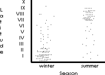
Changes are often more complex than the simple dichotomous changes with dichotomous causal factors, just illustrated. The complex case can be easily illustrated by changing the example to the migration of birds. The first figure below illustrates a dichotomous change in the number of birds in North and South America between the dichotomous periods of winter and summer. Each dot could represent some millions of birds.
Changes can also be continuous like dawn rather than dichotomous like a room light. Changes can be statistical like the percentage of birds in each location. Not all need fly south. 100% can be in Canada and 0% in South America or the reverse or anything in between. In fact, the birds may stop in the US, Panama, or anywhere in between or some could even migrate backwards.
This next figure illustrates most, but not all, elements in the dependent variable (dots or birds) "switching" with a change in the dichotomous independent variable (season).
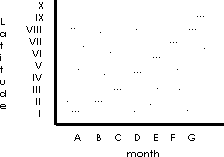
Further, it can be seen that change can be continuous in both its x and y amount. This is illustrated by plotting the data as a function of both all twelve months (A through G) and all ten latitudes (I through X) which gives us a more typical and more useful example.
The previous format provided for:
Time A through G
x
x
(location of birds) I through X
x
x
Illustrated in the following figure
x
x
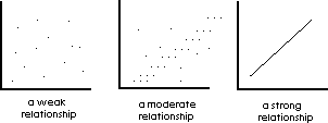
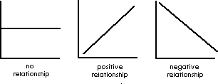
Not only do we get continuous x and y, but we can also get weak or strong relationships and positive or negative relationships.
The following variations of a scatter plot illustrate:
Clearly a single dependent variable can change as the result of more than one independent variable. In fact, it may not change unless several variables are manipulated in a particular way. Additionally, a single independent variable may cause several dependent variables to change. In this light, the previous examples can be seen as special cases of what changes we could expect in the natural world. The earlier examples have only one independent variable and one dependent variable; they are called univariate. The multivariate nature of the natural world has gotten lost because analysis simplifies in order to understand things and the analytical tools for multivariate analysis have only recently become available. In the past, all statistics were univariate.
Ball on a plane.
Ball in a valley, pendulum at bottom.
iii. Unstable Equilibrium
Pendulum at top.
iv. Metastable Equilibrium
Ball pushed into next valley.
The previous section on covariance skipped around a relatively complex issue without drawing attention to it. The issue however must be dealt with. Rarely do we find two subjects with exactly the same score. Rarely does an individual behave in an absolutely identical fashion from one occasion to the next occasion of the same situation. We must have a responsible way to treat this variation. We must have a truthful and coherent way to understand why behavior varies.
If we were to accept that all things were randomly determined, we could easily "explain" any differences in our dependent variables, we could say "it just happened that way for no reason," but we would cease to productively function. If things have no cause, how are we to predict, control, synthesize, and explain? As a matter of principle, we must assume that things occur for a reason, and that we can understand that reason. We, therefore, must presume that any difference in our measure is the result of different deterministic causes.
At a more practical level however, we will also have to accept that the deterministic source of the variation is sometimes beyond our resolving power. We get things handed to us like the distribution of electrons in any single atomic shell. The dilemma is that if we accept randomness at the broadest level, science ceases -- everything is simply random. If two children score differently on a test, nothing could be understood or done about it. On the other hand, if we require absolutely no variance in our measures, science will also cease because we would never get a clear answer to an experiment.
The solution is that the individual researcher is obliged to attack the major sources of variance in the phenomena of interest first, and report stability and accountable variance of the same magnitude as other researchers in the field. In a sense, status in science goes to the researchers who have the least variability in their data. Any difference between subjects (or between different instances with the same subject) is presumed to be the result of deterministic differences between those subjects or those situations. Research explains the variability by demonstrating covariance with the cause and no covariance without the cause. An initial step in the answer to the question of why the birds are sometimes in Argentina and sometimes in Canada is discovering the way the scores could be grouped (e.g., treatment, no treatment; or group 1 versus group 2) such that accountable variance is maximized. In the migrating birds example, it would be to group the dependent variable by season or by month. Most of the variability would then be accounted for by the time of year. The differences in the subjects can be conceptualized as occurring at a variety of levels (e.g. chemical, biological, psychological) or as the result of experiences across a variety of time scales (e.g. evolution, developmental, learning). These frameworks were developed in detail in the last chapter. Variance is said to be accounted for when we know how and why the scores vary. It is said to be residual when we don't understand why.
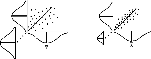
Like height and IQ, or height and weight, different degrees of relationship could occur. For example suppose we go around a typical class and ask each person for their height and IQ and we plot the left scatter plot below. We go up the Y-axis their height then across the X axis their IQ. We place a dot in that spot to represent that a person with that height and that IQ occurred. We notice that there are more people of average height than very tall or very short. This could be seen by imagining that each dot is a ball bearing and we tilt the page to the left. If the bearings roll straight to the left they would form stacks against the Y-axis as is illustrated. There would be many in the middle, few to the top or bottom. We can of course do the same with IQ along the X-axis. Many would be in the middle and few to the left or right. Next we repeat the whole plotting process by asking each person for their height and weight and form the right figure below. Again there are more middle height people than tall or short. There are also more middle weight people than light or heavy.

Note that the variability around the average Y (height) is the same in both figures (as it should be), and the variability around the average X is the same in both figures. However, in the right figure we could find a way of looking at the figure (in this case up the line drawn at a 45 degree angle) which dramatically reduces the error or variance around a central tendency. This is illustrated by the distribution drawn in the lower left corner of the figure. This error is very much smaller than that on the X or Y axis. If we had tilted the figure at a 45 degree angle than the stacks of ball bearings would have been very close together and would have created the distribution in the lower left corner.
The figure on the left has the same spread around the x and y axes, but it does not have any "line" around which the spread is minimized. A 45 degree line is drawn but clearly the spread around it is the same as around the mean x or y. If we know a person's height, we cannot accurately predict their IQ, whereas if we know their height, we could predict their weight. As can be seen on the left, prediction is not possible with a zero relationship. No information is available at all; whereas with the strong relationship on the right, accurate predictions can be made. This requires four elements: change on the "X" dimension; change on the "Y" dimension; reduced variability around the regression line as compared to around the mean; and sufficient spread in the elements on each axis.
This can be illustrated yet another way. Each circle below represents the variability in a set of numbers. The area of the circle labeled Y represents the variability on the Y-axis. The area of the circle labeled X represents the variability on the X-axis. The intersection of the two circles represents the covariance while the area in Y remaining in addition to the overlap represents the variability around the regression line or the variability in Y not "explained" or accounted for by the variability in X.
a. Models of Accountable Variance
There are several types of models for accountable variance. They differ with respect to what is known, or what information is specified by the model, and the certainty of their predictions.
It is necessary to experimentally manipulate the relevant variables to prove that a cause-effect relationship exists.
Some things, like a billiard ball moving as the result of being hit by the cue ball can be seen in a cause-effect framework where each step in the process is well understood. A light switch and room illumination is another example. (Manipulation ’ change; known reductionistic mechanism of action.) What steps and processes led to the end?
Things often stabilize in predictable ways without us understanding (or caring about) the reductionistic processes involved. Planets stabilize at known speeds and positions, water runs down to the sea, the rate of responding changes in orderly ways when the reinforcement rate changes, and so on. It helps little to explain celestial mechanics by saying that an unspecifiable force causes it or the rate changed because the animal knew something. Newton said "I have not been able to discover the (reductionistic) cause and I make no hypotheses." In this case explanation is only ordering sense data. (Manipulation ’ changes; unknown reductionistic mechanism of action, but known order of effect).
Some times we only know that things go together. One thing is not known to cause the other. Additionally, we may not even know which comes first. Social respectability and wealth covary. One can be predicted from the other but one does not force the other. Any of three relationships could underlie the prediction. It could be A ’ B; B ’ A; or C ’ A and B. (No manipulation; predictor ’ predicted with unknown order of effect.) (Experimental research could find order of effect.)
When we have discovered why something happens, we have removed the accountable variance. The next question is obviously what to do with the variability which we do not understand.
The obvious and productive solution to the problem of residual variability in the data from the subjects is to ask "why?" Why do these individuals score higher, how can I predict which of the scores will be higher? What will change an individual? By manipulating variables, you can find the answer.
b. Assumption of Nonlinear Dynamics
There are ways for a few simple completely deterministic variables to interact such that the result is a seemingly random series of measures (chaos theory). The resulting variations cannot always be proven nonrandom by simply observing the output. By developing a model of the processes underlying the behavior those factors could be resolved. It should be noted however that without the "deencryp-tion key," this interpretation is purely metaphysical. Without some coherent and broadly-based theoretical framework and substantial empirical support for a particular nonlinear dynamical causal factor, “chaos” is not an explanation.
c. Assumption of "True Score" and "Random Error"
While not properly a solution, this approach allows the researcher to "pass" on the problem. A property of randomness is that deviations occur to either side of a true score to the same extent. The mean of random errors cancel. If we presume that our obtained scores are randomly distributed around a true score then the mean will be the true score. If we have unaccounted for variability in our data, we can presume that it is random and of no interest by taking the average of our scores. This is covered in more detail in Chapter 5. However, we are: 1) presuming something which we do not know, 2) ignoring something which may be of importance, 3) assuming that each subject is identical and that its function is linear (it is more likely that each subject's function varies with respect to its parameters), and 4) each time you average data you are giving up opportunities to explain variability. Undoubtedly some variability should be passed over. It is equally true however, that some variability is of great consequence.
What appears to be a simple solution to residual variability is the “tag team solution.” When faced with a problem which, for you, is insurmountable, do like the wrestler does: Rush over to the ropes (the boundary of your domain) and give the problem to someone else. This would be contending that there is a biological explanation for your psychological data or a developmental explanation for your obtained difference in learning. These deferrals are different from experimental solutions because the investigator who invokes them does not pursue the problem across the boundary, but rather lays it at someone else’s doorstep and then acts as if the problem is understood by using the invoked paradigm as an explanation rather than a description of ignorance. Passing an unsolved problem to someone else is a mark of inadequacy, not a badge of honor.


Date Last Reviewed: November 17, 2002


