Behavior Changes over Time

Behavior changes over time. Our task is to understand it. The first step is to be able to describe it; the second step is to be able to predict it.

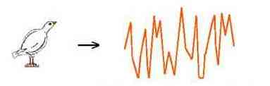
	distribution of the operant in time

Conceptualizations for Behavior

In the past, the task of understanding behavior change was simplified to only describing and predicting the overall behavior, or mean of many momentary measures of behavior. For example, "On average the rate doubled when the condition was changed from A to B" or "The asymptotic rate to this schedule was 2.4 responses per second." (Where the dependent variable was the mean rate during five, 1 hour sessions following 25 or more sessions of exposure to the procedures.) These types of measures are labeled "static".

If there were 240 pecks in a 4 minute window as illustrated, the response rate would be 1 peck per second with either order.

The future task of behavior analysis is to understand the moment to moment changes in behavior. These types of measures are labeled "dynamical" and must be displayed in two dimensions. A single number cannot characterize them.

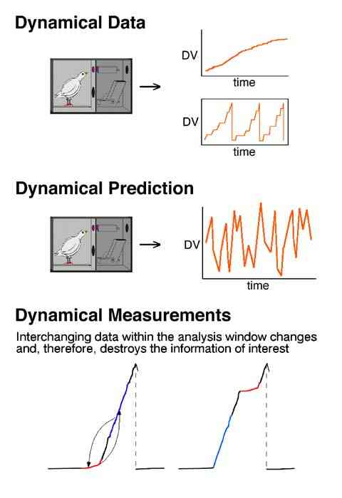
In the first case a high response rate follows a low response rate; in the second case the high rate precedes the low rate.

Behavioral Dynamics and Terminology

There are three broad categories of behavioral dynamics. Historical examples of their study have been fixed-interval performance (synchronous), the learning curve (transient), and "noise" (asynchronous).

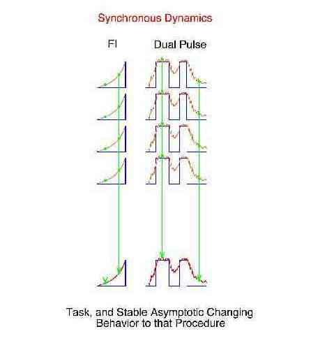
A "synchronous dynamic" is the common behavior change across some specific repeating procedure. It is obtained by determining the mean for the first bin and the mean for the second bin, and so on. The bins are in a fixed position with respect to some anchor point within each repetition of the procedure. These bin means are referred to a "synchronous means" or "repeated trial local averages". Signal averagers determine the synchronous dynamics following some synchronizing event such as a light flash to the eye. The synchronous dynamical measure is thought to be the best estimate of the effect of the procedure because the noise has been removed by taking the mean of many samples.

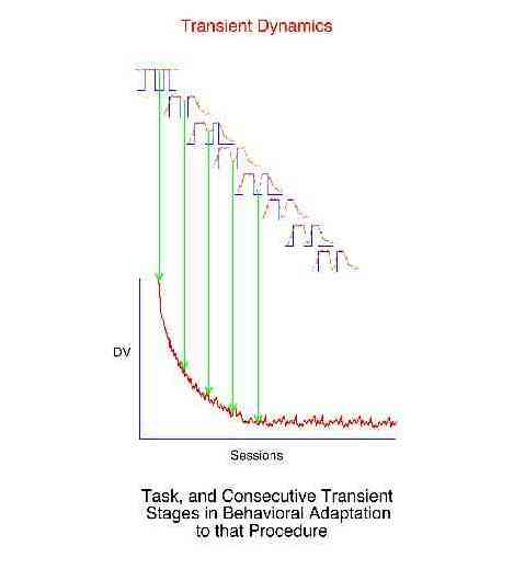
Transient dynamics refer to the "one time" behavioral adjustment to a change in conditions. The learning curve is an example of transient dynamics. Transient dynamics cannot be signal averaged because the essence of the effect is the change in behavior with each successive repetition of the task. The behavioral adjustment to the 500th exposure to a task is predictably different from the first exposure. Transient dynamics are not synchronous dynamics in that synchronous dynamics refer to what is the same about the behavior change to repetitions of a task, while transient dynamics refer to the systematic change in behavior with increasing experience with the task. Transient dynamics are unlike simple noise because given the specific starting point the behavior is very predictable and not at all random.

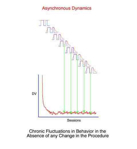
Asynchronous dynamics are those behavior changes which are random. Specific points in the behavior stream cannot be found which would allow principled synchronous averaging, i.e. the behavior cannot be easily attributed to some change in the environment.

An Analytical Approach to Dynamical Behavior

There are a number of possible approaches to take when trying to study behavioral dynamics. The following analysis is a special case of filter analysis and requires simplifying assumptions and constraints. They were accepted for the most part in order to:

1. Take advantage of a very well established analytical technology used in other disciplines to understand changing output,

2. Simplify the task enough so that some progress could be made.

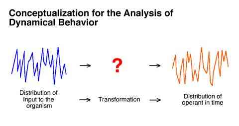
The first assumption is depicted in the following figure. It is simply the view that the output of an organism can be attributed to the input to that organism. Specifically, that some principled transformation can be carried out on some properties of the input to an organism which will result in correct predictions of some properties of the output from the organism.

In the present case:

1. Both the input and output can be seen as changing frequencies.

2. The moment to moment pattern of an organism's response rate changes are assumed to be attributable to the moment to moment pattern of obtained reinforcement rate changes.

3. Each frequency component of the input and output is seen as totally independent of all other frequencies,

4. The entire effect of the organism can be characterized as amplifying or attenuating specific input frequencies.

5. The function relating output to input is constant for an individual across various learning histories and across procedure changes.

These assumptions maximally simplify the analytical task and are the defining properties of linear analysis.

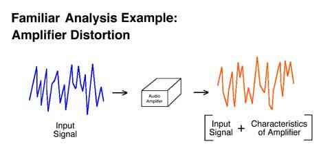
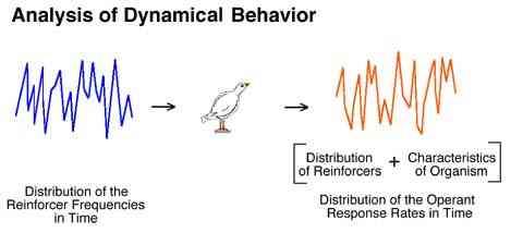
We are very familiar with this approach when we consider audio amplifiers. The inputs to and outputs from an animal can be conceptualized similarly. The specific pattern of moment to moment changes in the reinforcement rate is thought to control the specific pattern of moment to moment changes in the response rate.

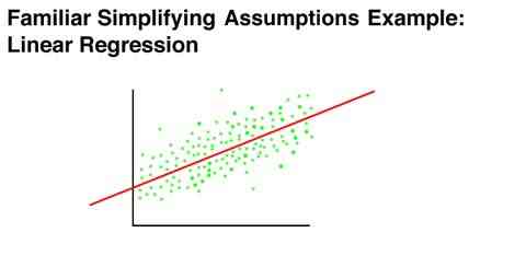
The simplifying assumptions of linear analysis are very similar to the assumptions underlying linear regression. Linear regression assumes that the true regression is the same at all points, and that the regression does not change as the result of what immediately precedes a particular point on the x axis. It is obvious that linear regression does not capture every relationship known to exist, and in fact is not always the most perfect index in the situation in which it is used. It is also apparent that linear regression has been a very productive tool in psychology

To the degree that these constraints of linear analysis are true, then a family of well understood analysis techniques can be used as powerful tools to understand the dynamic aspects of behavior. The great power of this type of analysis is that it will predict a zero free parameter output for any possible input. It will specify the precise filter characteristics for a particular organism which will predict the precise output given any possible input.

It is important to note that this is not to say that any conceivable behavioral process is in fact totally characterized by linear analysis (any more than linear regression makes an analogous claim). Rather the value in linear analysis and linear regression is in their ability to characterize a useful portion of the variance in the data, by making the assumptions that they do.

Linear Analysis of Dynamical Behavior

1. The Logic underlying the Machinery of Linear Analysis

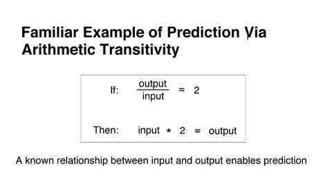
The logic underlying the mathematical machinery of these analyses is very simple and is familiar to everyone.

First, predictions can be made based on arithmetic transitivity. If you have previously determined that the output is twice the input, for example, then given the input you can predict that the output will be twice as large.

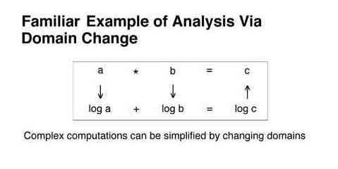
Second, many computations can be simplified by changing domains. For example, rather than multiplying two numbers to determine a prediction, it is often easier to convert the original numbers to their logs, add the logs, and find the antilog of the sum.

2. The Steps Involved in Linear Analysis

The following figure depicts virtually all of the important machinery of the present research. It shows how the relationship between a known input and a known output can be used to predict a dynamical output given a known input.

The function (illustrated in green) used to adjust any given input in order to predict an output is labeled a "transfer function."

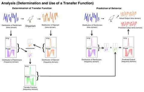
The upper left section of the figure depicts the conversion of the pattern of the reinforcers in the reinforcer pulse input and the resulting response rates into the frequency domain and the division of each of the output frequencies (and phases) by their respective input frequencies (and phases). The quotient is the transfer function; it specifies how each frequency was changed by the organism. The upper right section depicts some arbitrary reinforcement pattern input, its conversion to the frequency domain and that representation multiplied by the transfer function, which corrects each frequency for the distortion which is expected to be added by the organism. This produces the frequency domain representation of the predicted output. This is then converted to the time domain and compared to the actual output of the bird, bin by bin, to determine the quality of the prediction.

3. The Experimental Procedure Enabling Linear Analysis

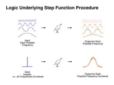
The following experimental procedure dramatically simplifies the determination of an animal's transfer function. Recall the conceptual similarity in the relationship between an input and an output of an animal and the input and output of an audio amplifier. If behavior is to be predicted for any possible frequency input, then the "distortion" for each possible input frequency must be empirically determined. This is obviously a daunting task. However, a simplifying realization can be made. Fourier's theorem shows that an impulse could be seen as containing all possible frequencies of sine waves. As a result, if a single impulse is presented to an audio amplifier, or an organism, that is in effect presenting all possible frequencies (all at once) the output will therefore also contain all possible frequencies (all at once) plus any "distortion" added to each of those frequencies. In other words, an impulse input every hour will reveal how the system will react to any and all possible frequencies between a few seconds and an hour.

Because a zero duration pulse cannot be implemented and a short pulse of VI is used. An imperfect sample of all possible frequencies is obtained. Some frequencies will be missed resulting in an imperfect transfer function, but the example procedure is a reasonable first approximation.

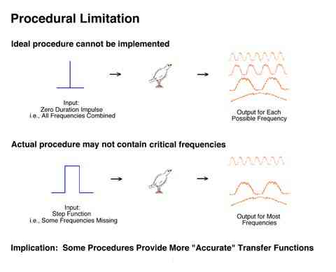
The simplest procedure which could be used to determine an animal's transfer function is to present reinforcers in the form of a short reinforcement period or pulse. A transfer function covering the frequencies of greatest interest (i.e., behavior changes which take place more often than once per hour) can be approximated with a procedure providing extinction for a few minutes followed by a VI schedule for a few minutes followed by extinction for a few minutes, such that the entire cycle is about 1 hour in duration. A constant anchor point to start the interval could be provided with a blackout. This type of schedule is labeled a "pulse procedure".

4. The Procedural Implications of the Assumptions Underlying Linear Analysis

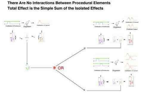
The assumed constancy of an organism's transfer function has several implications with respect to the validity of experimental procedures. It implies that the behavior resultant of any pattern of inputs is independent of all other inputs. This independence refers to:

1. Independence from schedule

2. Independence from prior history

3. Independence from interaction of component procedures

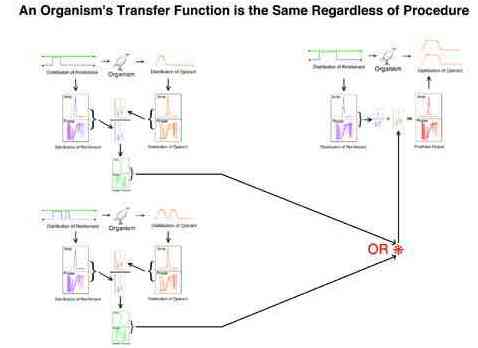
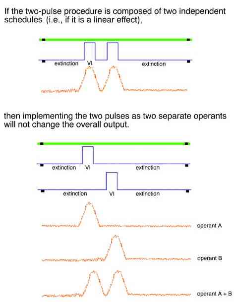
For example, in principal the transfer function obtained from a one or a two pulse procedure predicts the behavior to a novel long pulse procedure equally well.

For example, in principal the transfer function obtained from a particular procedure is the same regardless of prior exposure to a long or very long pulse procedure.

For example, in principal a transfer function can predict the output of a two pulse procedure regardless of whether those two pulses are implemented on one or on two keys.

Implications of Linear Analysis

Because the organism is conceptualized as a "filter" it gives us a way to understand one of the most fundamental questions in the analysis of behavior. (Recall that in the general case a filter can amplify a frequency as well as simply attenuate it.)

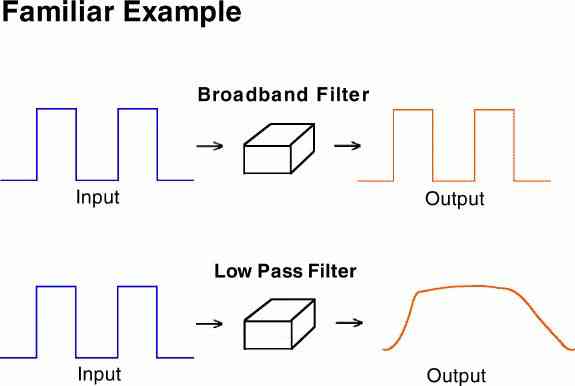
A broad-band filter passes all the details (both sharp edges and slow trends) of the input signal. An audio amplifier is better if it passes all of these details. A low pass filter on the other hand, would blur all the fine details and give only the broad averages. A very inexpensive or low fidelity amplifier is said to have a poor "frequency response" because of its poor band pass characteristics.

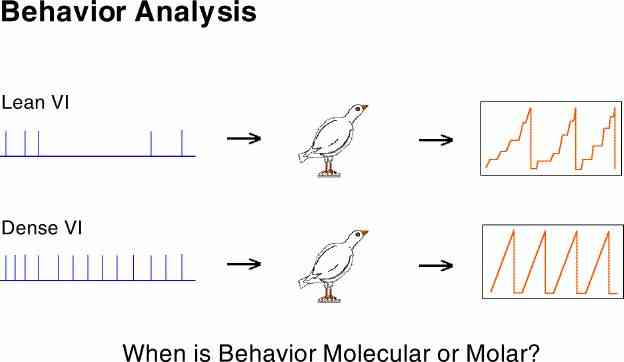
An important aspect of the behavior of organisms is the degree to which it follows all the small transitions in the contingencies of reinforcement or the degree to which is smoothes over the fine details. The most obvious example of smoothing over changes in the input is provided by the behavior under a VI schedule. Even though there are periods of reinforcers far apart as well as close together, the organism has a steady output. This is illustrated in the bottom section of the above illustration. This difference in responsiveness to the details in the contingencies of reinforcement has been labeled "molecular" (reacts to small changes) and "molar" (does not react to small changes).

This difference can be more usefully seen as the filter characteristics of the organism (e.g., broad-band versus low-pass). The importance of this relabeling is that it connects us to an enormous body of conceptual and analytical tools used to great benefit by "older" sciences.

The Original Research Applying Linear Analysis to Behavior

Palya, Walter, Kessel, & Lucke (1996)

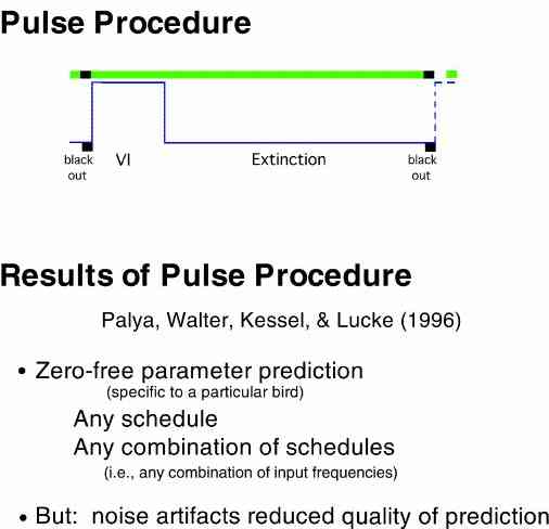
It was shown that reasonable, zero-free parameter predictions could be made based on the use of a transfer function obtained with this procedure. It is important to reiterate that no scaling adjustments are used with this method. It is truly a zero free parameter prediction.

While it was shown that the conceptual machinery would work, the predictions were not perfect. Our subsequent research in this area was intended to further reduce the error of prediction caused by noise by developing better experimental procedures and better analytical and numerical methods.

Advancements in the Analysis Technique

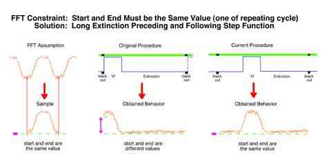
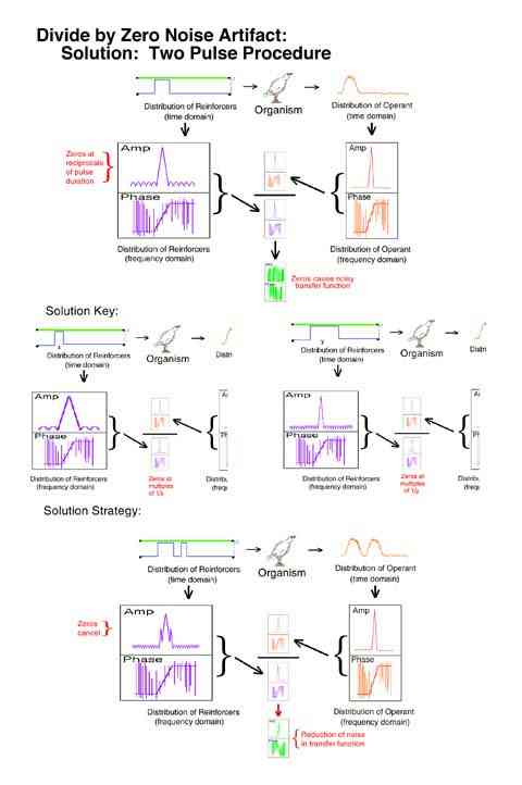
Because of the novelty of this research program, a number of relatively simple but important procedural optimizations were revealed. First, if Fourier transforms are to be accomplished using FFT algorithms, then several constraints must be met. One of which is that one complete segment of a continuing pattern must be used. This requires that the response rate at the beginning of a trial must approximate the response rate at the end of the trial. Our original procedure of signaling each trial start with a blackout and providing the pulse at the beginning of the trial lead to a high response rate at the start of the trial. This implied that behavior would show a virtually zero duration ramp up to an unsignaled pulse which was clearly false.

A second problem uncovered was that a single pulse procedure resulted in a mathematical artifact. The analysis produced no information at all at reciprocals of the pulse duration. This was equivalent to a situation where the size of a microphone caused a dead spot at all harmonics of a particular note. A foot long microphone would be dead for C sharp for example. This artifact would necessarily delete C sharp from every octave in a piece of music. The solution would be to use two microphones of different sizes and combine their output. The solution in the present case was to use a two pulse procedure where the two pulses were of different durations. What the first pulse could not detect the second pulse filled in.

Potential Noise Reduction Techniques

One problem with linear analysis has been its less than ideal signal-to-noise ratios. It would be expected that a more aggressive averaging procedure would increase the signal-to-noise ratio. The view was that larger samples would diminish random error and averaging in both the time and frequency domain would maximally reduce noise. We evaluated a procedure which first averaged across large samples (20 day averages), then averaged those five samples in the frequency domain (the transfer functions) to produce a best estimate of the "true" transfer function.

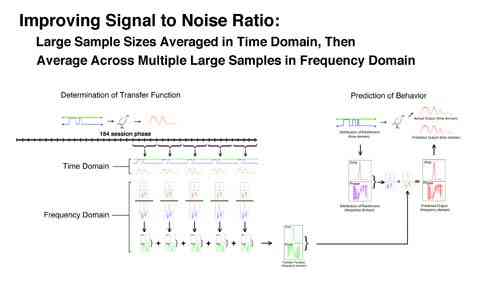
Our current solution is to no longer allocate so much of the spectrum to behaviorally impossible frequencies. We are no longer sampling at an extremely high rate which "detects" substantial amounts of high frequency noise and then subsequently attempt to remove that noise with complex numerical methods. By analogy, rather than measuring the time of pecks to the picosecond (which results in substantial artifactual variability in the peck times) and then smoothing down to milliseconds, we are measuring peck times to the nearest millisecond. It is simply not meaningful to emphasize picosecond variability if pecks were to occur exactly 38 milliseconds apart.

Research Evaluating Advanced Linear Analysis

Palya, Walter, Kessel, & Luke (2000)

Results of the offset double pulse procedure:

Development of a better experimental procedure to determine the transfer function.

Procedure

Results

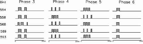
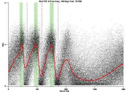
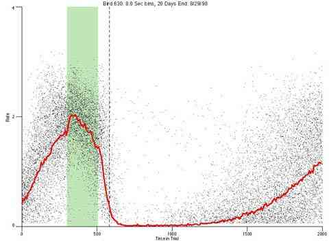
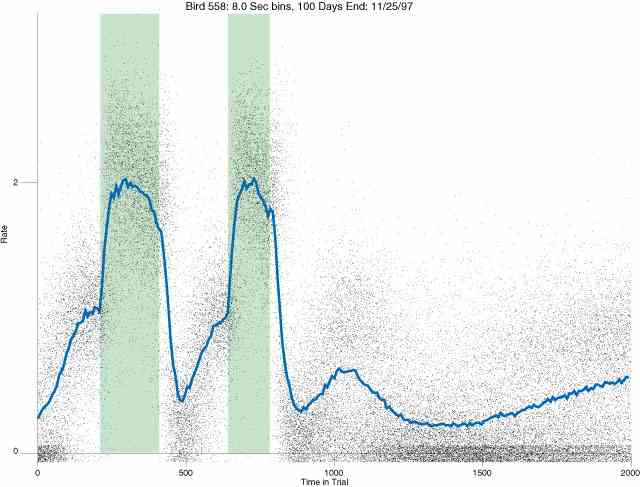
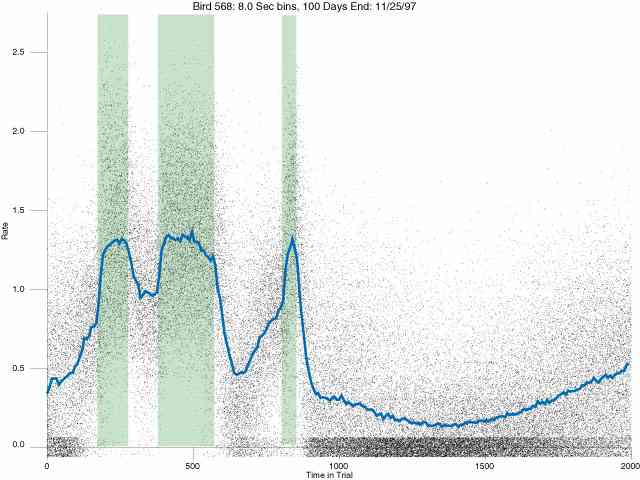
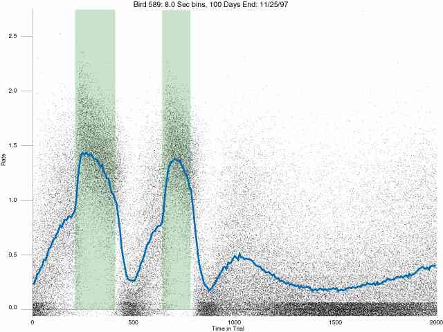
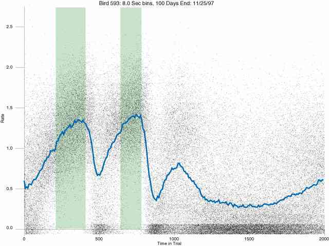
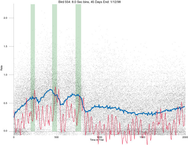
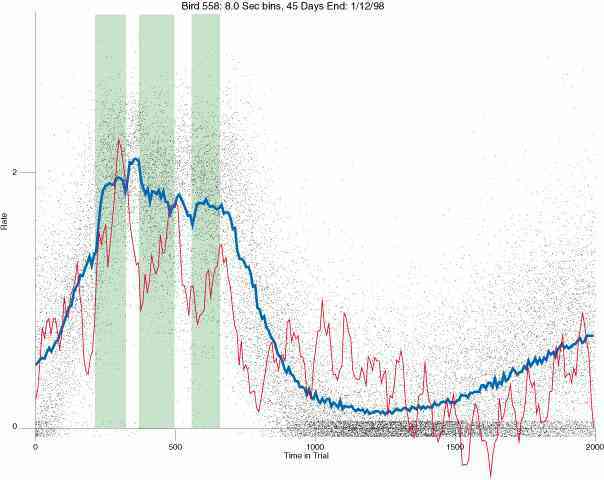
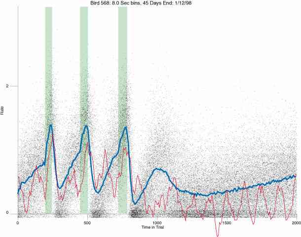
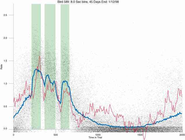
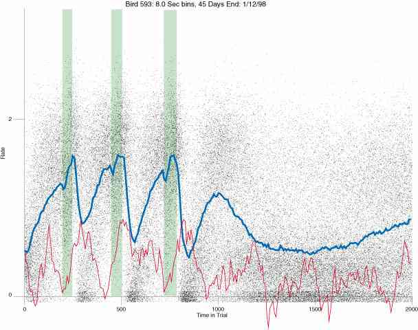
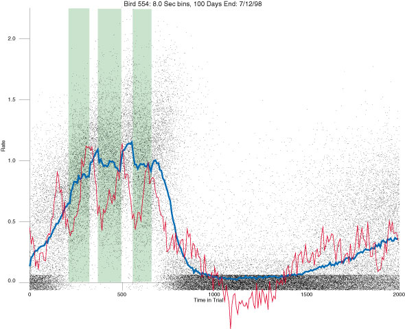
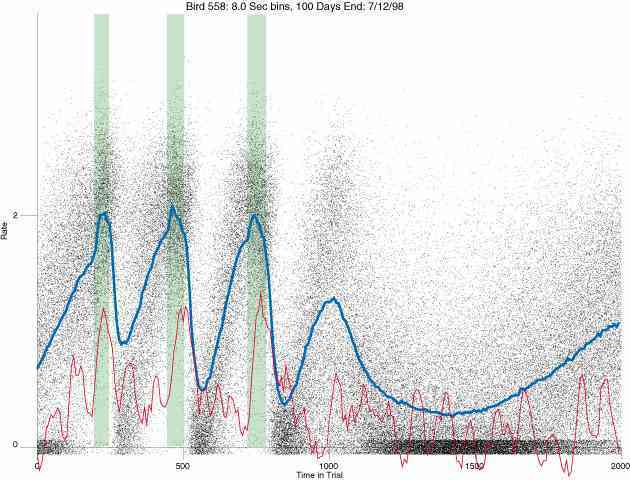
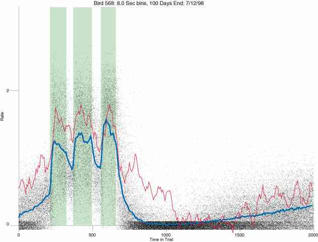
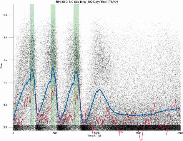
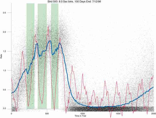
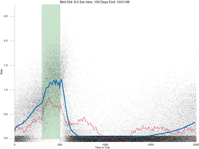
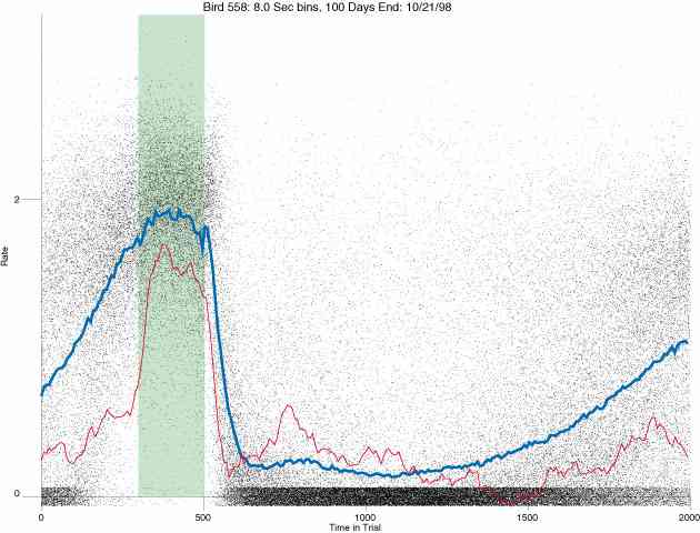
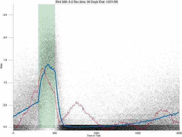
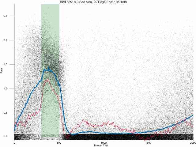
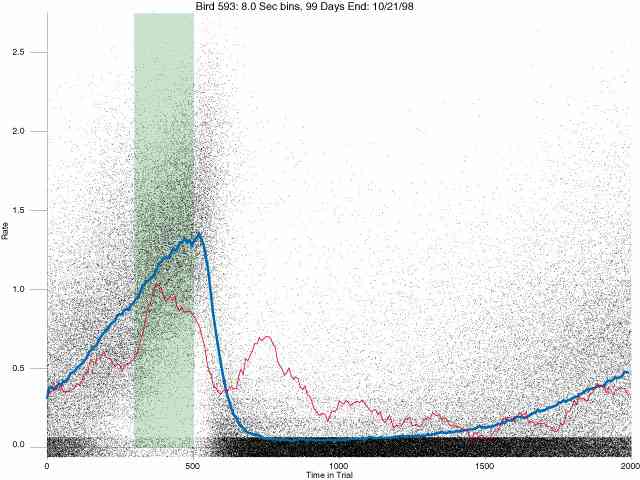
In the following dot plots the trial duration is represented across the X axis. The heavy blue function depicts the mean rate in each portion of the trial. The red function depicts the predicted mean rate generated by linear analysis. The green bars depict the portion of the interval containing the VI-20 schedule. Each dot in the frame represents the rate for an 8 second bin for one trial, for that position in the trial. By noting the relative density of dots the modal behavior for each portion of the trial can easily be discerned. Additionally the dispersion of behavior is also clearly depicted.

Because only a quantal number of pecks could occur in each 8 second bin thus producing quantal rates, and because a single quantal columns of data one dot wide would represent the responding across each 8 second bin; the dot representing the response rate for each bin was dithered on the x-axis (± 1/2 bin) and on the y-axis (± 1/2 peck per 8 second bin). This portrayal therefore assumes that responding is spread equally across the 8 second bin and that response rates are continuous. The width of the dithering on the y-axis can be seen by noting the vertical dithering of the dots representing zero pecks in an 8 second bin. They are plotted ± 1/2 peck per 8 second bin on either side of the x-axis.

The following figures portray the response rate every 8 seconds throughout the trial for 100 sessions.

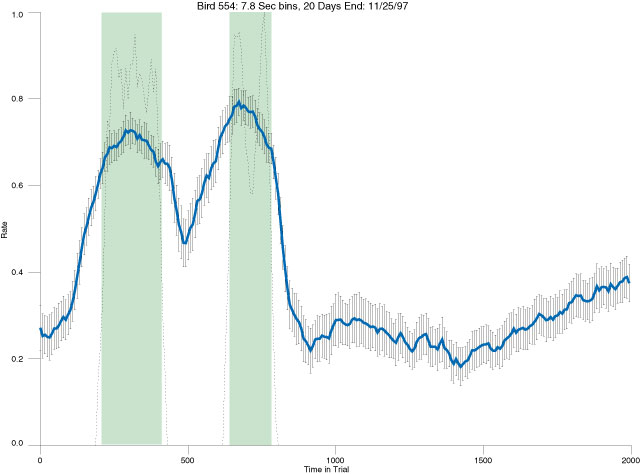
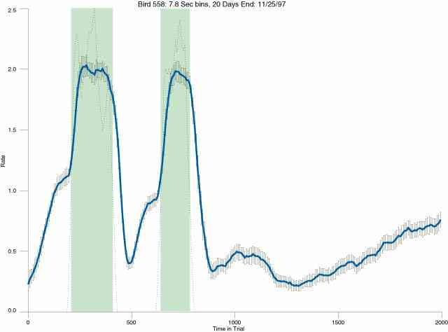
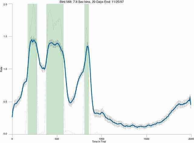
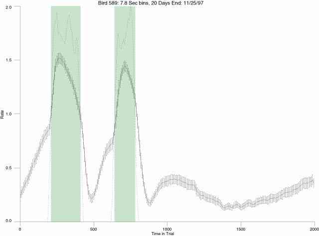
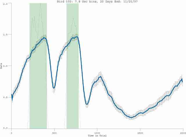
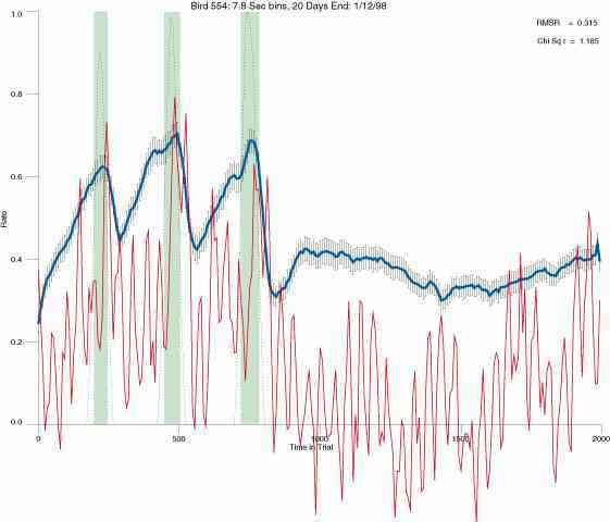
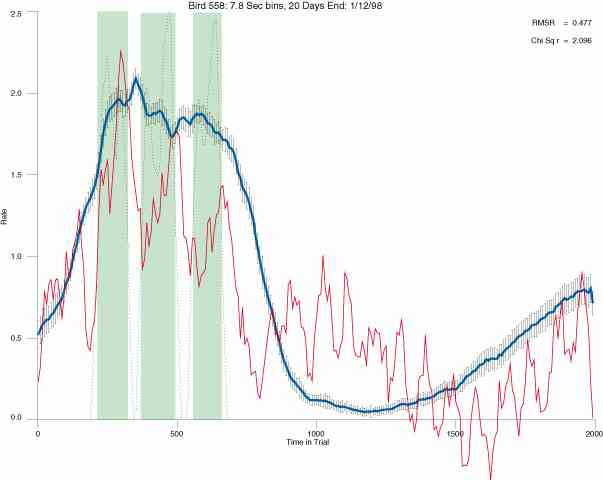
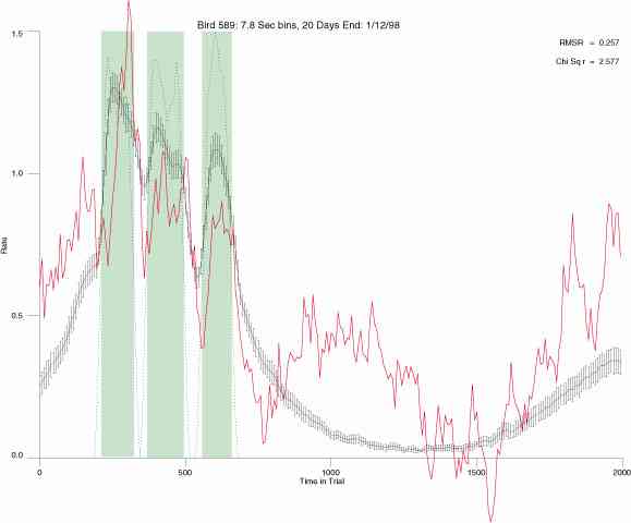
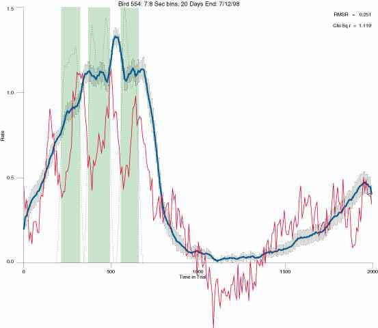
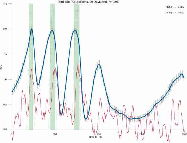
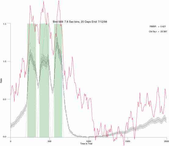
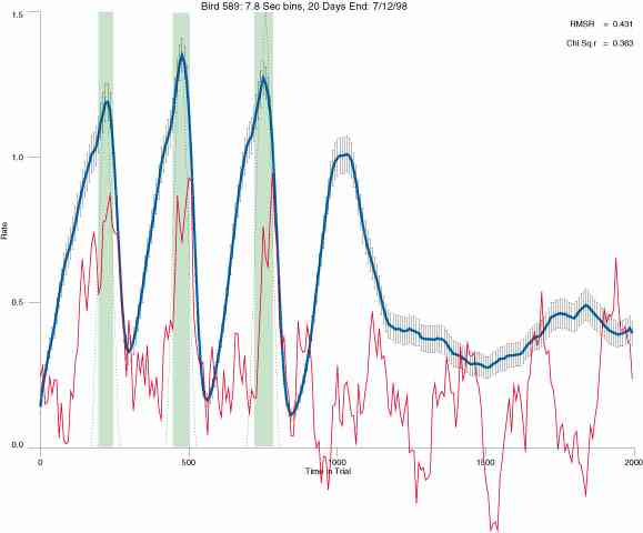
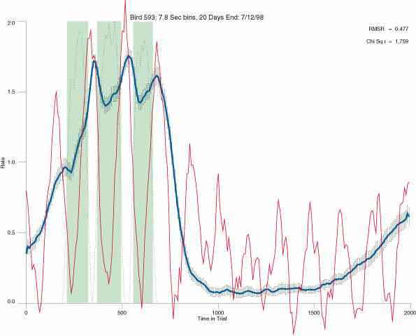
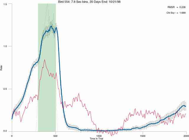
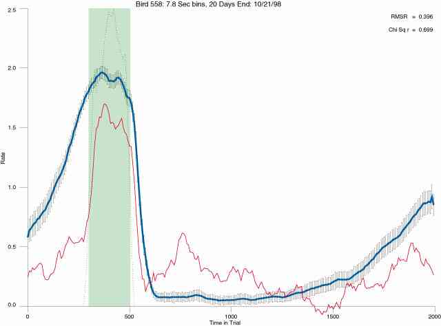
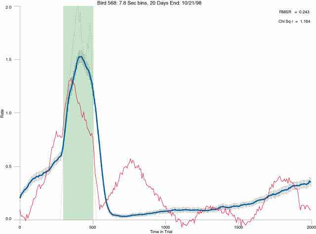
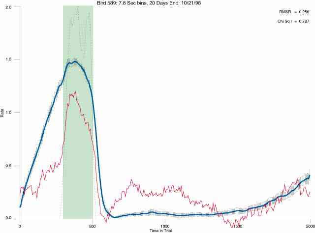
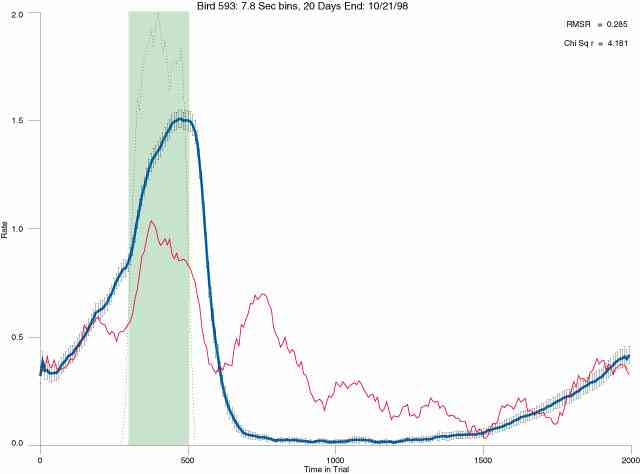
The following figures portray the mean response rate in each portion of the trial (blue function) (the same information as was provided by the blue function in the earlier set of frames). The standard error of the mean (as calculated by dividing the standard deviation of the data points in each 8 second bin by the square root of the sample size) is depicted by the whiskers. The standard error of the mean in each bin is a function of the vertical spread of the dots in that bin as is shown in the preceding set of frames. The predicted rate generated by linear analysis is given by the red function. This function is identical to the red function in the earlier set of frames. The dotted functions depict the obtained reinforcement rate in each 8 second bin throughout the trial. The green bars depict the portion of the interval containing the VI-20 schedule. The quality of the fit as indexed by reduced chi square (Chi Sq r) as well as the root mean squared residual (RMSR) is provided in the upper right of each frame.

The following figures are animations of how the response rate across the trial changed from trial to trial. By running the animation the trial by trial behavior dynamics can be observed. The common behavior change across the trial across the phase is labeled synchronous dynamics. The change in the behavior change across the early exposure to the procedure is labeled "transient dynamics". The unsystematic changes in the behavior from trial to trial are labeled "asynchronous dynamics". The sliding average animations portray a 5 day sliding window of the same data and portrays the changes in the measure most typically used to portray static data (i.e. the mean of the last 5 days for a phase). It removes a substantial amount of the asynchronous dynamics.

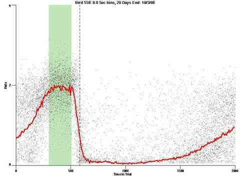
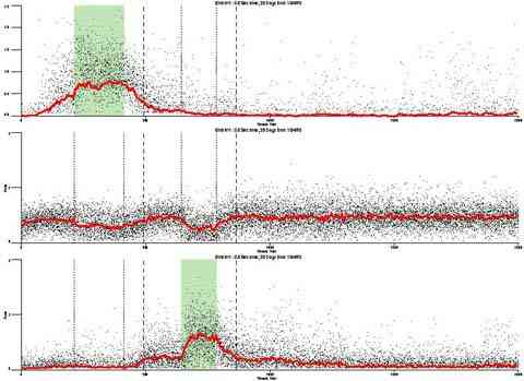
As an alternate visualization example the following 3 dimensional color projection plots show the distribution of response rates across the trial obtained during the last 20 days of Phase 5 for bird 558.

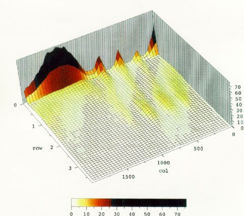
The X axis shows the time in trial where the beginning of the trial is on the right. The Y axis shows the response rate, and the Z axis and color index show the probability of rate occurance.

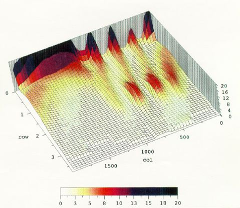
The second figure reduces the Z axis range to facilitate viewing the smaller changes in rate without being swamped by the large peak at a 0 rate.

All predictions were bases on the Phase 3 data. Two predictions were generated for each bird for each of phases 4,5, and 6. The predictions were based on either one sample (20 sessions) or on 5, 20 session samples who's transfer functions had been averaged (note that the data was resampled in the analysis program and the resultant predictions were 256 elements long.

The data table contains:

1. The input and output for each bird under; the last 20 sessions, and the last 5 20 session samples under phase 3 (the 5th sample of the 5 sample set is identical to the single sample).
2. The input and output data files for each bird for each of phases 4, 5, and 6
3. A prediction for each bird in each phase based on the single sample and the MatLab program used to carry out the analysis.
4. A prediction for each bird in each phase based on the 5 sample data and the MatLab program used to carry out the analysis.

			Bird 554	Bird 558	Bird 568	Bird 589	Bird 593
Phase 3	1 Sample	Obtained	Input Variance Output Variance	Input Variance Output Variance	Input Variance Output Variance	Input Variance Output Variance	Input Variance Output Variance
	5 Samples	Obtained	Input1 Input2 Input3 Input4 Input5 Output1 Output2 Output3 Output4 Output5	Input1 Input2 Input3 Input4 Input5 Output1 Output2 Output3 Output4 Output5	Input1 Input2 Input3 Input4 Input5 Output1 Output2 Output3 Output4 Output5	Input1 Input2 Input3 Input4 Input5 Output1 Output2 Output3 Output4 Output5	Input1 Input2 Input3 Input4 Input5 Output1 Output2 Output3 Output4 Output5
Phase 4		Obtained	Input Variance Output Variance	Input Variance Output Variance	Input Variance Output Variance	Input Variance Output Variance	Input Variance Output Variance
	1 Sample	Predict	Prediction	Prediction	Prediction	Prediction	Prediction
		Program	P3 to P4	P3 to P4	P3 to P4	P3 to P4	P3 to P4
	5 Samples	Predict	Prediction	Prediction	Prediction	Prediction	Prediction
		Program	P3 to P4	P3 to P4	P3 to P4	P3 to P4	P3 to P4
Phase 5		Obtained	Input Variance Output Variance	Input Variance Output Variance	Input Variance Output Variance	Input Variance Output Variance	Input Variance Output Variance
	1 Sample	Predict	Prediction	Prediction	Prediction	Prediction	Prediction
		Program	P3 to P5	P3 to P5	P3 to P5	P3 to P5	P3 to P5
	5 Samples	Predict	Prediction	Prediction	Prediction	Prediction	Prediction
		Program	P3 to P5	P3 to P5	P3 to P5	P3 to P5	P3 to P5
Phase 6		Obtained	Input Variance Output Variance	Input Variance Output Variance	Input Variance Output Variance	Input Variance Output Variance	Input Variance Output Variance
	1 Sample	Predict	Prediction	Prediction	Prediction	Prediction	Prediction
		Program	P3 to P6	P3 to P6	P3 to P6	P3 to P6	P3 to P6
	5 Samples	Predict	Prediction	Prediction	Prediction	Prediction	Prediction
		Program	P3 to P6	P3 to P6	P3 to P6	P3 to P6	P3 to P6

The meaningfulness of filter analysis with respect to the description and prediction of the behavior of organisms is not yet fully established. There are certainly many hopeful signs, but there are also some quite thorny problems.

The first issue is how well will filter analysis ultimately describe and predict behavior in specialized test cases. This depends on development in two areas.

1. The development of better analytical procedures which will deal with factors missed by a simple linear analysis
   1. Other filter techniques such as Butterworth filters
   2. The integration of a non-linear term to linear analysis
2. The development of better experimental procedures which reveal the nature of the processes which are not captured by linear analysis. Correctly modeling these additional processed is an essential element to progress in filter analysis

The second issue is how well will a filter analysis

1. Capture some important aspect of behavior so that it can be removed analytically. In that way a researcher need only focus attention on some additional process of interest. This is analogous to removing the linear component from regression so that only the higher order relationship can be studied.
2. Predict into new procedures and be useful in producing behavior with specific properties. For example, the researcher may wish to produce a sag in responding with specific parameters at a specific point in the schedule. The analysis should be able to provide the schedule parameters which will produce that behavior.

Our current research addresses several of these issues

Experimental Analysis: Removal of Additional Processes

The Determinants of the Rate Increase Across the Trial

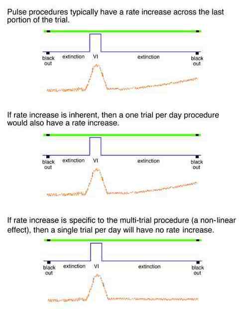
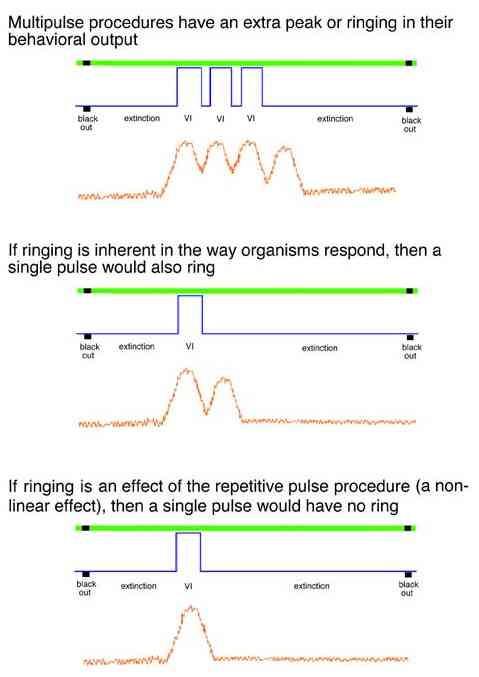
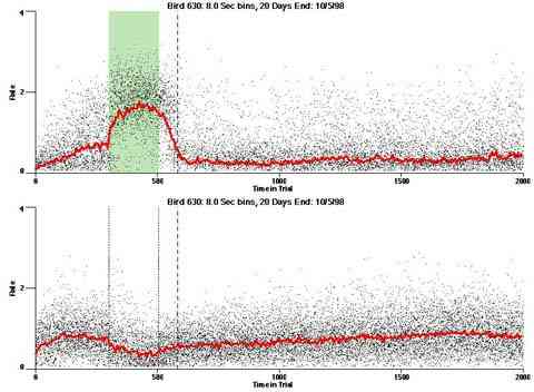
As implemented, the multi trial procedure with a VI schedule pulse generates a slow increase across the latter half of each trial. This could be an anticipatory rise in rate controlled by the upcoming reinforcement pulse or it could be an intrinsic effect of the prior reinforcement pulse. Exposing the birds to a single trial per day would eliminate the anticipatory rise if it were a higher-order effect.

Logic

Empirical Test

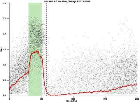
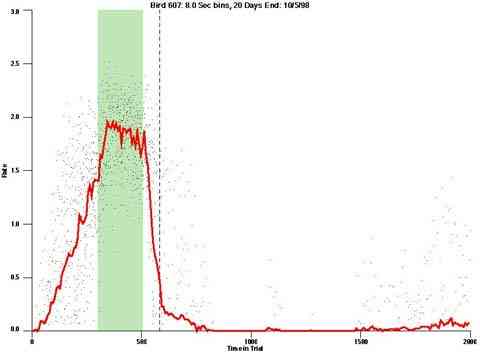
The dotted line in the dot plot designates "+1 Max IRI" it designates the elapse of the longest IRI if it had been initiated at the end of the VI pulse period. If behavior were under the control of the time since the prior reinforcer it is the worst case "confirmed-end-of-pulse".

Determinants of the Behavioral "Ringing"

Typically multipulse procedures generate an increase in rate as if there were one more reinforcement pulse in the procedure.

Logic

Empirical Test

Determinants of the "Operant Noise"

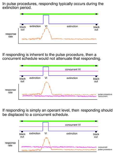
As implemented, the pulse procedure also generates a background rate of responding. This effect suggests that the responding shows less precise stimulus control than it would if responding were more costly or if some other concurrent activity were competing with the behavior to the pulse procedure.

Logic

Empirical Test

Evaluation of the Independence of Effect

A linear analysis also predicts that two schedule pulses occurring on separate keys is exactly the same as two pulses on the same key. Linear analysis argues that the behavioral result of a procedure has no dependence on what the organisms experiences before, after, or at the same time.

Logic

Empirical Test

Experimental Synthesis: Production of Desired Behavior

Demonstration of an Inverse Solution

An example of the practical and paradigmatic fecundity of a model of behavior is its ability to provide the tools to solve inverse questions. An example would be "what separation in pulses (or reinforcement rate) are necessary to cause a 50% decrement in rate?" Alternatively, "what width of a pulse (or reinforcement rate) would produce a 50% increment in rate?" To the degree that linear analysis can provide a general framework for these questions, it will contribute to a systematic account for them.

Logic

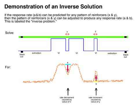
Two procedures were used to solve the "inverse problem".

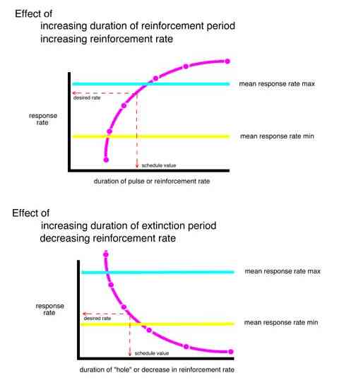
In the trial and error forward procedure the pulse separation which would result in the desired mean relative response rate (50%) in the first interpulse interval was found by predicting outputs for a range of schedule parameters and then interpolating the parameters to find the separation which would produce the desired results. The reinforcement rate required to produce the desired response rate (50%) during the third pulse was similarly interpolated.

The predicted behavior for each bird (based on that bird's transfer function) to each of five hypothetical schedules with increasingly larger extinction periods and to each of five hypothetical schedules with increasingly thin VI schedules were determined. A curve was fit to the increasing and decreasing series for each bird. The schedule which would produce a 50% sag in the behavior and the reinforcement rate within a pulse which would produce a 50% rise in the behavior was determined for each bird.

Determination of Schedule Values

The results of this procedure are not yet available.

In the second procedure a true inverse solution was determined.

The logic of the procedure was to first select a general pattern across the 8000 sec trial that was likely to be an attainable pattern for pigeons. The desired pulse width and spacing parameters were based on the actual behavior of a bird to a pilot procedure which roughly produced the desired 50% sag and 50% rise in behavior. This desired square wave output was transformed to the frequency domain and divided by the transfer function for each bird. The result was then converted back to the time domain to produce the necessary input pattern for that bird which would produce the desired output pattern.

The results of this procedure are not yet available.

Date Last Modified : October 6, 2003